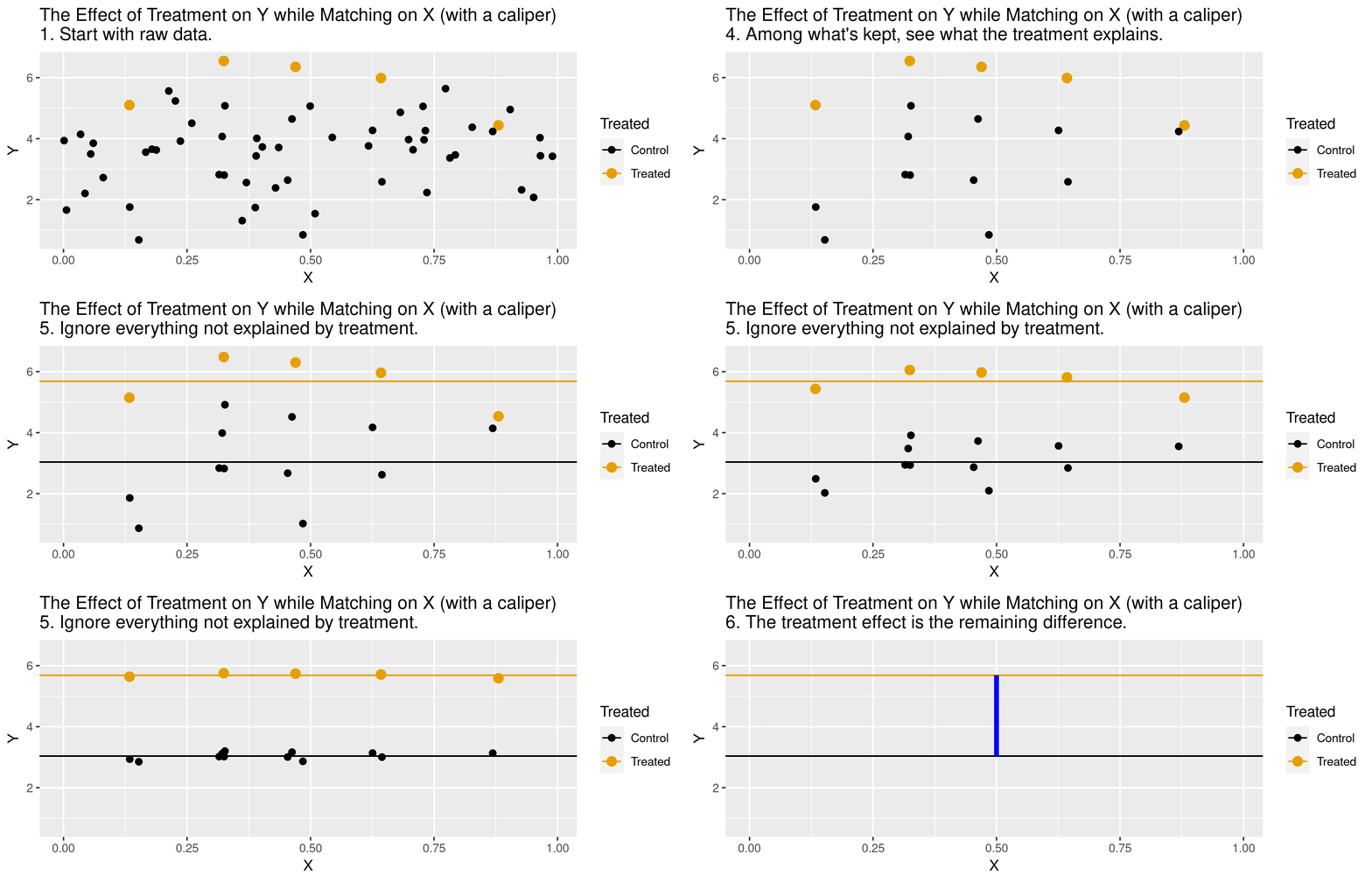
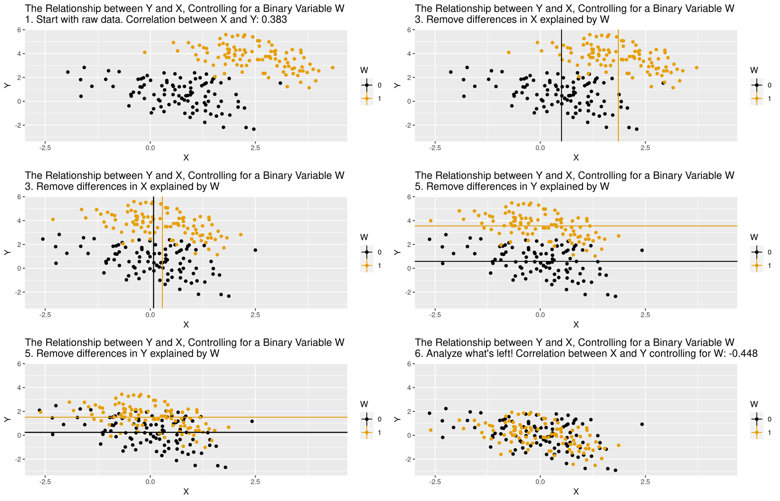
Module 1: Hospital Pricing and Selection on Observables

class: center, middle, inverse, title-slide

.title[
# Module 1: Hospital Pricing and Selection on Observables
]
.subtitle[
## Part 2: Matching and Weighting
]
.author[
### Ian McCarthy | Emory University
]
.date[
### Econ 470 & HLTH 470
]

---

<style type="text/css">
.remark-slide-content {
 font-size: 30px;
 padding: 1em 2em 1em 2em; 
}
.remark-code {
 font-size: 15px;
}
.remark-inline-code { 
 font-size: 20px;
}
</style>

# Goal

Find covariates `$X_{i}$` such that the following assumptions are plausible:

1. Selection on observables: `$$Y_{0i}, Y_{1i} \perp\!\!\!\perp D_{i} | X_{i}$$`
2. Common support: `$$0 < \text{Pr}(D_{i}=1|X_{i}) < 1$$`

Then we can use `$X_{i}$` to group observations and use expectations for control as the predicted counterfactuals among treated, and vice versa.

---
# Assumption 1: Selection on Observables

`$E[Y_{1}|D,X]=E[Y_{1}|X]$`

In words...nothing unobserved that determines treatment selection and affects your outcome of interest.

---
# Assumption 1: Selection on Observables

- Example of selection on observables from *Mastering Metrics*

---
# Assumption 2: Common Support
Someone of each type must be in both the treated and untreated groups

--
`$$0 < \text{Pr}(D=1|X) <1$$`

---
# Causal inference with observational data

With selection on observables and common support:

1. Subclassification
2. Matching estimators
3. Reweighting estimators
4. Regression estimators

---
# Subclassification

Sum the average treatment effects by group, and take a weighted average over those groups:

`$$ATE=\sum_{i=1}^{N} P(X=x_{i}) \left(E[Y | X, D=1] - E[Y | X, D=0]\right)$$`

---
# Subclassification

- Difference between treated and controls
- Weighted average by probability of given group (proportion of sample)
- What if outcome is unobserved for treatment or control group for a given subclass?

- This is the *curse of dimensionality*

---
# Matching: The process
1. For each observation `$i$`, find the `$m$` "nearest" neighbors, `$J_{m}(i)$`. 
2. Impute `$\hat{Y}_{0i}$` and `$\hat{Y}_{1i}$` for each observation: 
`$$\hat{Y}_{0i} = \begin{cases}
 Y_{i} & \text{if} & D_{i}=0 \\
 \frac{1}{m} \sum_{j \in J_{m}(i)} Y_{j} & \text{if} & D_{i}=1 
\end{cases}$$`
`$$\hat{Y}_{1i} = \begin{cases}
 Y_{i} & \text{if} & D_{i}=1 \\
 \frac{1}{m} \sum_{j \in J_{m}(i)} Y_{j} & \text{if} & D_{i}=0 
\end{cases}$$`

3. Form "matched" ATE: 
`$\hat{\delta}^{\text{match}} = \frac{1}{N} \sum_{i=1}^{N} \left(\hat{Y}_{1i} - \hat{Y}_{0i} \right)$`

---
# Matching: Defining "nearest"

1. Euclidean distance: 
`$\sum_{k=1}^{K} (X_{ik} - X_{jk})^{2}$`

2. Scaled Euclidean distance: 
`$\sum_{k=1}^{K} \frac{1}{\sigma_{X_{k}}^{2}} (X_{ik} - X_{jk})^{2}$`

3. Mahalanobis distance: 
`$(X_{i} - X_{j})' \Sigma_{X}^{-1} (X_{i} - X_{j})$`

---
# Animation for matching

.center[
  ![:scale 900px](pics/match_animate.gif)
]

---
# Matching: Defining "nearest"

- But are observations really the same in each group?
- Potential for "matching discrepancies" to introduce bias in estimates

- "Bias correction" based on `$$\hat{\mu}(x_{i}) - \hat{\mu}(x_{j(i)})$$` (i.e., difference in fitted values from regression of `$y$` on `$x$`, with the difference between observed `$Y_{1i}$` and imputed `$Y_{0i}$`)

---
# Weighting

1. Estimate propensity score `ps <- glm(D~X, family=binomial, data)`, denoted `$\hat{\pi}(X_{i})$`
2. Weight by inverse of propensity score 
.center[
`$\hat{\mu}_{1} = \frac{ \sum_{i=1}^{N} \frac{Y_{i} D_{i}}{\hat{\pi}(X_{i})} }{ \sum_{i=1}^{N} \frac{D_{i}}{\hat{\pi}(X_{i})} }$` and 
`$\hat{\mu}_{0} = \frac{ \sum_{i=1}^{N} \frac{Y_{i} (1-D_{i})}{1-\hat{\pi}(X_{i})} }{ \sum_{i=1}^{N} \frac{1-D_{i}}{1-\hat{\pi}(X_{i})} }$`
]
3. Form "inverse-propensity weighted" ATE: 
.center[
`$\hat{\delta}^{IPW} = \hat{\mu}_{1} - \hat{\mu}_{0}$`
]

---
# Regression
1. Regress `$Y_{i}$` on `$X_{i}$` among `$D_{i}=1$` to form `$\hat{\mu}_{1}(X_{i})$`
2. Regress `$Y_{i}$` on `$X_{i}$` among `$D_{i}=0$` to form `$\hat{\mu}_{0}(X_{i})$`
3. Form difference in predictions: 
.center[
`$$\hat{\delta}^{reg} = \frac{1}{N} \sum_{i=1}^{N} \left(\hat{\mu}_{1}(X_{i}) - \hat{\mu}_{0}(X_{i})\right)$$`
]

---
# Regression

Or estimate in one step, 
.center[
`$$Y_{i} = \delta D_{i} + \beta X_{i} + D_{i} \times \left(X_{i} - \bar{X}\right) \gamma + \varepsilon_{i}$$`
]

- Note the `$(X_{i} - \bar{X})$`. What does this do?

---
# Animation for regression

.center[
  ![:scale 900px](pics/reg_animate.gif)
]

---
# Simulated data
Now let's do some matching, re-weighting, and regression with simulated data:

```r
n <- 5000
select.dat <- tibble(
 x = runif(n, 0, 1),
 z = rnorm(n, 0, 1),
 w = (x>0.65),
 y = -2.5 + 4*w + 1.5*x + rnorm(n,0,1),
 w_alt = ( x + z > 0.35),
 y_alt = -2.5 + 4*w_alt + 1.5*x + 2.25*z + rnorm(n,0,1)
)
```

---
# Simulation: nearest neighbor matching

```r
nn.est1 <- Matching::Match(Y=select.dat$y,
 Tr=select.dat$w,
 X=select.dat$x,
 M=1,
 Weight=1,
 estimand="ATE")
summary(nn.est1)
```

```
## 
## Estimate...  3.8785 
## AI SE......  0.53145 
## T-stat.....  7.298 
## p.val......  2.9199e-13 
## 
## Original number of observations..............  5000 
## Original number of treated obs...............  1731 
## Matched number of observations...............  5000 
## Matched number of observations  (unweighted).  5013
```

---
# Simulation: nearest neighbor matching

```r
nn.est2 <- Matching::Match(Y=select.dat$y,
 Tr=select.dat$w,
 X=select.dat$x,
 M=1,
* Weight=2,
 estimand="ATE")
summary(nn.est2)
```

---
# Simulation: regression

```r
reg1.dat <- select.dat %>% filter(w==1)
reg1 <- lm(y ~ x, data=reg1.dat)

reg0.dat <- select.dat %>% filter(w==0)
reg0 <- lm(y ~ x, data=reg0.dat)
pred1 <- predict(reg1,new=select.dat)
pred0 <- predict(reg0,new=select.dat)
mean(pred1-pred0)
```

```
## [1] 4.126236
```

---
# Violation of selection on observables
.pull-left[
NN Matching

```r
nn.est3 <- Matching::Match(Y=select.dat$y_alt,
 Tr=select.dat$w_alt,
 X=select.dat$x,
 M=1,
 Weight=2,
 estimand="ATE")
summary(nn.est3)
```

```
## 
## Estimate... 7.6502 
## AI SE...... 0.053248 
## T-stat..... 143.67 
## p.val...... < 2.22e-16 
## 
## Original number of observations.............. 5000 
## Original number of treated obs............... 2756 
## Matched number of observations............... 5000 
## Matched number of observations (unweighted). 22555
```
]

.pull-right[
Regression

```r
reg1.dat <- select.dat %>% filter(w_alt==1)
reg1 <- lm(y_alt ~ x, data=reg1.dat)

reg0.dat <- select.dat %>% filter(w_alt==0)
reg0 <- lm(y_alt ~ x, data=reg0.dat)
pred1_alt <- predict(reg1,new=select.dat)
pred0_alt <- predict(reg0,new=select.dat)
mean(pred1_alt-pred0_alt)
```

```
## [1] 7.675315
```
]

---
# What covariates to use?

- There are such things as "bad controls"
- We want to avoid control variables that are:

- Outcomes of the treatment
- Also endogenous (more generally)