Introduction to Causal Inference

Ian McCarthy | Emory University

Outline for Today

1. Overview of Class
2. Intro to Causal Inference
3. Potential Outcomes
4. Average Treatment Effects

Class Overview

Why this course?

1. Major problems that need solutions
2. Need good, convincing empirical work for policy
3. Working with data is hard, particularly health care data
4. Your work should be transparent and reproducible

Structure

• Very applied in nature
• Methods for causal inference
  • Selection on observables (regression, re-weighting, matching, propensity scores)
  • Instrumental variables
  • Regression discontinuity
  • Difference-in-differences

Structure

• Substantive areas
  • Hospital pricing, policy, and competition
  • Medicare Advantage and quality disclosure
  • Medicaid expansion and health insurance

Structure

• Datasets from the real world
  • Hospital Cost Report Information System (HCRIS)
  • Medicare Advantage data

Assignments

• Homework (x5)
• Peer Reviews (x5)

Grading

Component	Weight
5 × homework assignments (15% each)	75%
5 x peer review (5% each)	25%

Introduction to Causal Inference

Motivating question

Let’s motivate things with this simple question…does health care spending improve our health?

Spending and Health

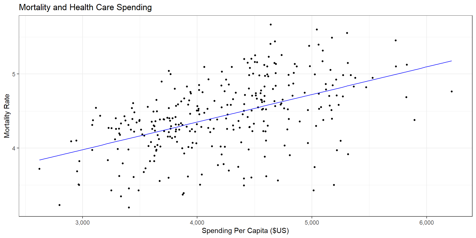
ggplot(data = (dartmouth.data %>% filter(Year==2015)), 
       mapping = aes(x = Expenditures, y = Total_Mortality)) + 
  geom_point(size = 1) + theme_bw() + scale_x_continuous(label = comma) +
  geom_smooth(method="lm", se=FALSE, color="blue", size=1/2) +
  labs(x = "Spending Per Capita ($US)",
       y = "Mortality Rate",
       title = "Mortality and Health Care Spending")

Spending and Health

• Does medical spending make us sicker?
• What else might explain this relationship?

Why causal inference?

Another example: What price should we charge for a night in a hotel?

Machine Learning

• Focuses on prediction
• High prices are strongly correlated with higher sales
• Increase prices to attract more people?

Causal Inference

• Focuses on counterfactuals
• What would sales look like if prices were higher?

Goal of Causal Inference

• Goal: Estimate effect of some policy or program
• Key building block for causal inference is the idea of potential outcomes

The Potential Outcomes Framework

Notation

Treatment \(D_{i}\)

\[D_{i}=\begin{cases} 1 \text{ with treatment} \\ 0 \text{ without treatment} \end{cases}\]

Notation

Potential outcomes

• \(Y_{1i}\) is the potential outcome for unit \(i\) with treatment
• \(Y_{0i}\) is the potential outcome for unit \(i\) without treatment

Notation

Observed outcome

\[Y_{i}=Y_{1i} \times D_{i} + Y_{0i} \times (1-D_{i})\] or

\[Y_{i}=\begin{cases} Y_{1i} \text{ if } D_{i}=1 \\ Y_{0i} \text{ if } D_{i}=0 \end{cases}\]

Assumes SUTVA (stable unit treatment value assumption)…no interference across units

Example of “Potential Outcomes”

\(Y_{1}\)= $75,000

\(Y_{0}\)= $60,000

Single-year earnings due to Emory = \(Y_{1}-Y_{0}\) = $15,000

Example of “Potential Outcomes”

\(Y_{1}\)= $75,000

\(Y_{0}\)= ?

Earnings due to Emory = \(Y_{1}-Y_{0}\) = ?

Do we ever observe the potential outcomes?

Without a time machine…not possible to get individual effects.

Fundamental Problem of Causal Inference

• We don’t observe the counterfactual outcome…what would have happened if a treated unit was actually untreated.
• ALL attempts at causal inference represent some attempt at estimating the counterfactual outcome. We need an estimate for \(Y_{0}\) among those that were treated, and vice versa for \(Y_{1}\).

Average Treatment Effects

Different treatment effects

Tend to focus on averages:

• ATE: \(\delta_{ATE} = E[ Y_{1} - Y_{0}]\)
• ATT: \(\delta_{ATT} = E[ Y_{1} - Y_{0} | D=1]\)
• ATU: \(\delta_{ATU} = E[ Y_{1} - Y_{0} | D=0]\)

or similar measures such as medians or quantiles

Average Treatment Effects

• Estimand: \[\delta_{ATE} = E[Y_{1} - Y_{0}] = E[Y | D=1] - E[Y | D=0]\]
• Estimate: \[\hat{\delta}_{ATE} = \frac{1}{N_{1}} \sum_{D_{i}=1} Y_{i} - \frac{1}{N_{0}} \sum_{D_{i}=0} Y_{i},\] where \(N_{1}\) is number of treated and \(N_{0}\) is number untreated (control)
• With random assignment and equal groups, inference/hypothesis testing with standard two-sample t-test

Selection bias

• Assume (for simplicity) constant effects, \(Y_{1i}=Y_{0i} + \delta\)
• Since we don’t observe \(Y_{0}\) and \(Y_{1}\), we have to use the observed outcomes, \(Y_{i}\)

\[\begin{align} E[Y_{i} | D_{i}=1] &- E[Y_{i} | D_{i}=0] \\ =& E[Y_{1i} | D_{i}=1] - E[Y_{0i} | D_{i}=0] \\ =& \delta + E[Y_{0i} | D_{i}=1] - E[Y_{0i} | D_{i}=0] \\ =& \text{ATE } + \text{ Selection Bias} \end{align}\]

Selection bias

• Selection bias means \(E[Y_{0i} | D_{i}=1] - E[Y_{0i} | D_{i}=0] \neq 0\)
• In words, the potential outcome without treatment, \(Y_{0i}\), is different between those that ultimately did and did not receive treatment.
• e.g., treated group was going to be better on average even without treatment (higher wages, healthier, etc.)

Selection bias

• How to “remove” selection bias?
• How about random assignment?
• In this case, treatment assignment doesn’t tell us anything about \(Y_{0i}\) \[E[Y_{0i}|D_{i}=1] = E[Y_{0i}|D_{i}=0],\] such that \[E[Y_{i}|D_{i}=1] - E[Y_{i} | D_{i}=0] = \delta_{ATE} = \delta_{ATT} = \delta_{ATU}\]

Selection bias

• Without random assignment, there’s a high probability that \[E[Y_{0i}|D_{i}=1] \neq E[Y_{0i}|D_{i}=0]\]
• i.e., outcomes without treatment are different for the treated group

Omitted variables bias

• In a regression setting, selection bias is the same problem as omitted variables bias (OVB)
• Quick review: Goal of OLS is to find \(\hat{\beta}\) to “best fit” the linear equation \(y_{i} = \alpha + x_{i} \beta + \epsilon_{i}\)

Regression review

\[\begin{align} \min_{\beta} & \sum_{i=1}^{N} \left(y_{i} - \alpha - x_{i} \beta\right)^{2} = \min_{\beta} \sum_{i=1}^{N} \left(y_{i} - (\bar{y} - \bar{x}\beta) - x_{i} \beta\right)^{2}\\ 0 &= \sum_{i=1}^{N} \left(y_{i} - \bar{y} - (x_{i} - \bar{x})\hat{\beta} \right)(x_{i} - \bar{x}) \\ 0 &= \sum_{i=1}^{N} (y_{i} - \bar{y})(x_{i} - \bar{x}) - \hat{\beta} \sum_{i=1}^{N}(x_{i} - \bar{x})^{2} \\ \hat{\beta} &= \frac{\sum_{i=1}^{N} (y_{i} - \bar{y})(x_{i} - \bar{x})}{\sum_{i=1}^{N} (x_{i} - \bar{x})^{2}} = \frac{Cov(y,x)}{Var(x)} \end{align}\]

Omitted variables bias

• Interested in estimate of the effect of schooling on wages \[Y_{i} = \alpha + \beta s_{i} + \gamma A_{i} + \epsilon_{i}\]
• But we don’t observe ability, \(A_{i}\), so we estimate \[Y_{i} = \alpha + \beta s_{i} + u_{i}\]
• What is our estimate of \(\beta\) from this regression?

Omitted variables bias

\[\begin{align} \hat{\beta} &= \frac{Cov(Y_{i}, s_{i})}{Var(s_{i})} \\ &= \frac{Cov(\alpha + \beta s_{i} + \gamma A_{i} + \epsilon_{i}, s_{i})}{Var(s_{i})} \\ &= \frac{\beta Cov(s_{i}, s_{i}) + \gamma Cov(A_{i},s_{i}) + Cov(\epsilon_{i}, s_{i})}{Var(s_{i})}\\ &= \beta \frac{Var(s_{i})}{Var(s_{i})} + \gamma \frac{Cov(A_{i},s_{i})}{Var(s_{i})} + 0\\ &= \beta + \gamma \times \theta_{as} \end{align}\]

Removing selection bias without RCT

• The field of causal inference is all about different strategies to remove selection bias
• The first strategy (really, assumption) in this class: selection on observables or conditional indpendence

Intuition

• Example: Does having health insurance, \(D_{i}=1\), improve your health relative to someone without health insurance, \(D_{i}=0\)?
• \(Y_{1i}\) denotes health with insurance, and \(Y_{0i}\) health without insurance (these are potential outcomes)
• In raw data, \([Y_{i} | D_{i}=1] > E[Y_{i} | D_{i}=0]\), but is that causal?

Intuition

Some assumptions:

• \(Y_{0i}=\alpha + \eta_{i}\)
• \(Y_{1i} - Y_{0i} = \delta\)
• There is some set of “controls”, \(x_{i}\), such that \(\eta_{i} = \beta x_{i} + u_{i}\) and \(E[u_{i} | x_{i}]=0\) (conditional independence assumption, or CIA)

\[\begin{align} Y_{i} &= Y_{1i} \times D_{i} + Y_{0i} \times (1-D_{i}) \\ &= \delta D_{i} + Y_{0i} D_{i} + Y_{0i} - Y_{0i} D_{i} \\ &= \delta D_{i} + \alpha + \eta_{i} \\ &= \delta D_{i} + \alpha + \beta x_{i} + u_{i} \end{align}\]

ATEs versus regression coefficients

• Estimating the regression equation, \[Y_{i} = \alpha + \delta D_{i} + \beta x_{i} + u_{i}\] provides a causal estimate of the effect of \(D_{i}\) on \(Y_{i}\)
• But what does that really mean?

ATEs vs regression coefficients

• Ceteris paribus (“with other conditions remaining the same”), a change in \(D_{i}\) will lead to a change in \(Y_{i}\) in the amount of \(\hat{\delta}\)
• But is ceteris paribus informative about policy?

ATEs vs regression coefficients

• \(Y_{1i} = Y_{0i} + \delta_{i} D_{i}\) (allows for heterogeneous effects)
• \(Y_{i} = \alpha + \beta D_{i} + \gamma X_{i} + \epsilon_{i}\), with \(Y_{0i}, Y_{1i} \perp\!\!\!\perp D_{i} | X_{i}\)
• Aronow and Samii, 2016, show that: \[\hat{\beta} \rightarrow_{p} \frac{E[w_{i} \delta_{i}]}{E[w_{i}]},\] where \(w_{i} = (D_{i} - E[D_{i} | X_{i}])^{2}\)

ATEs vs regression coefficients

• Simplify to ATT and ATU
• \(Y_{1i} = Y_{0i} + \delta_{ATT} D_{i} + \delta_{ATU} (1-D_{i})\)
• \(Y_{i} = \alpha + \beta D_{i} + \gamma X_{i} + \epsilon_{i}\), with \(Y_{0i}, Y_{1i} \perp\!\!\!\perp D_{i} | X_{i}\)

\[\begin{align} \beta = & \frac{P(D_{i}=1) \times \pi (X_{i} | D_{i}=1) \times (1- \pi (X_{i} | D_{i}=1))}{\sum_{j=0,1} P(D_{i}=j) \times \pi (X_{i} | D_{i}=j) \times (1- \pi (X_{i} | D_{i}=j))} \delta_{ATU} \\ & + \frac{P(D_{i}=0) \times \pi (X_{i} | D_{i}=0) \times (1- \pi (X_{i} | D_{i}=0))}{\sum_{j=0,1} P(D_{i}=j) \times \pi (X_{i} | D_{i}=j) \times (1- \pi (X_{i} | D_{i}=j))} \delta_{ATT} \end{align}\]

ATEs vs regression coefficients

What does this mean?

• OLS puts more weight on observations with treatment \(D_{i}\) “unexplained” by \(X_{i}\)
• “Reverse” weighting such that the proportion of treated units are used to weight the ATU while the proportion of untreated units enter the weights of the ATT
• This is an average effect, but probably not the average we want