Matching and Weighting

Ian McCarthy | Emory University

Outline for Today

1. What is “Selection on Observables”?
2. Many different estimators
3. Practice with simulated data

Selection on Observables

Problem of “Selection”

Recall the selection or endogeneity problem:

• Estimand: \[\delta_{ATE} = E[Y_{1} - Y_{0}] = E[Y | D=1] - E[Y | D=0]\]
• Estimate: \[\hat{\delta}_{ATE} = \frac{1}{N_{1}} \sum_{D_{i}=1} Y_{i} - \frac{1}{N_{0}} \sum_{D_{i}=0} Y_{i},\] where \(N_{1}\) is number of treated and \(N_{0}\) is number untreated (control)

\[\hat{\delta}_{ATE} = \frac{1}{N_{1}} \sum_{D_{i}=1} Y_{i} - \frac{1}{N_{0}} \sum_{D_{i}=0} Y_{i}\]

• Since we don’t observe \(Y_{0}\) and \(Y_{1}\), we have to use the observed outcomes, \(Y_{i}\)

\[\begin{align} E[Y_{i} | D_{i}=1] &- E[Y_{i} | D_{i}=0] \\ =& E[Y_{1i} | D_{i}=1] - E[Y_{0i} | D_{i}=0] \\ =& \delta + E[Y_{0i} | D_{i}=1] - E[Y_{0i} | D_{i}=0] \\ =& \text{ATE } + \text{ Selection Bias} \end{align}\]

• Selection bias means \(E[Y_{0i} | D_{i}=1] - E[Y_{0i} | D_{i}=0] \neq 0\)

Clarification of terminology

• “Selection” or “self-selection” sometimes used to describe process of missing data (e.g., people “self-select” into the labor market)
• We’re using “selection” differently…captures process by which units are associated with specific values of covariates (e.g., in a study of hospital admits and health, patients are in the hospital because of unobserved things also related to their health)

Potential Solution…

Find covariates \(X_{i}\) such that the following assumptions are plausible:

1. Selection on observables: \[Y_{0i}, Y_{1i} \perp\!\!\!\perp D_{i} | X_{i}\]
2. Common support: \[0 < \text{Pr}(D_{i}=1|X_{i}) < 1\]

• KEY INTUITION: My potential outcomes are unchanged by treatment status…treatment status governs which potential outcome is observed in the data
• Then we can use \(X_{i}\) to group observations and use expected values from control group as the predicted counterfactuals among treated, and vice versa.

Assumption 1: Selection on Observables

\(E[Y_{1}|D,X]=E[Y_{1}|X]\)

In words…nothing else, outside of \(X\), that determines treatment selection and affects your outcome of interest.

Assumption 2: Common Support

Someone of each type must be in both the treated and untreated groups

\[0 < \text{Pr}(D=1|X) <1\]

Estimators Based on Selection on Observables Assumption

With selection on observables and common support:

1. Subclassification
2. Matching estimators
3. Reweighting estimators
4. Regression estimators

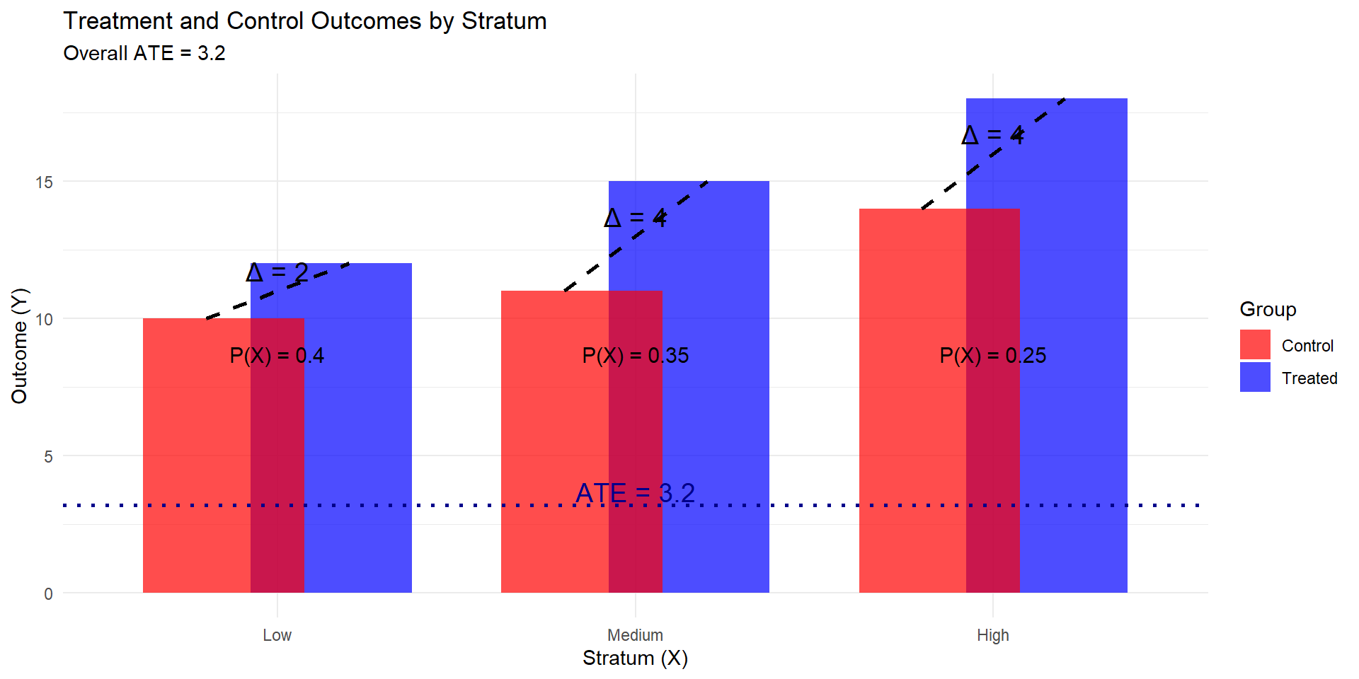
Subclassification

Sum the average treatment effects by group, and take a weighted average over those groups:

\[ATE=\sum_{i=1}^{N} P(X=x_{i}) \left(E[Y | X, D=1] - E[Y | X, D=0]\right)\]

Subclassification: Example

• Difference between treated and controls
• Weighted average by probability of given group (proportion of sample)

Stratum (X)	Proportion P(X)	Y (treated)	Y (control)	Treatment Effect	Contribution to ATE
Low	0.4	12	10	2	0.8
Medium	0.35	15	11	4	1.4
High	0.25	18	14	4	1.0

Final ATE Calculation: \[ATE = (0.4 \times 2) + (0.35 \times 4) + (0.25 \times 4) = 3.2\]

Subclassification: Graph

# Define the data with proportions
df <- data.frame(
  Stratum = factor(c("Low", "Medium", "High"), levels = c("Low", "Medium", "High")),
  P_X = c(0.4, 0.35, 0.25),  # Proportion of each stratum
  Treated = c(12, 15, 18),  
  Control = c(10, 11, 14)  
)

# Compute the ATE and per-group contributions
df <- df %>%
  mutate(TE = Treated - Control,  # Treatment effect per stratum
         Contribution = P_X * TE)  # Contribution to ATE

ATE <- sum(df$Contribution)  # Weighted sum

# Convert to long format for ggplot
df_long <- df %>%
  pivot_longer(cols = c("Treated", "Control"), names_to = "Group", values_to = "Outcome")

# Create the plot
ggplot(df_long, aes(x = Stratum, y = Outcome, fill = Group)) +
  
  # Bar plot for treated and control outcomes
  geom_bar(stat = "identity", position = position_dodge(width = 0.6), alpha = 0.7) +
  
  # Treatment effect slopes (dashed lines)
  geom_segment(data = df, aes(
    x = as.numeric(Stratum) - 0.2,  # Control (left)
    xend = as.numeric(Stratum) + 0.2,  # Treated (right)
    y = Control, 
    yend = Treated
  ), inherit.aes = FALSE, linetype = "dashed", color = "black", linewidth = 1) +
  
  # Slope labels (Δ = Treatment Effect)
  geom_text(data = df, aes(
    x = Stratum, 
    y = (Treated + Control) / 2,  # Middle of the dashed line
    label = paste0("Δ = ", TE)
  ), inherit.aes = FALSE, color = "black", vjust = -0.5, size = 5) +
  
  # Sample proportion labels (P(X) below bars)
  geom_text(data = df, aes(
    x = Stratum, 
    y = min(Control, Treated) - 1,  # Below the bars
    label = paste0("P(X) = ", P_X)
  ), inherit.aes = FALSE, color = "black", vjust = 1, size = 4) +

  # Horizontal ATE line
  geom_hline(yintercept = ATE, linetype = "dotted", color = "darkblue", linewidth = 1) +
  annotate("text", x = 2, y = ATE + 0.5, label = paste("ATE =", round(ATE, 2)), color = "darkblue", size = 5) +
  
  # Labels and theme
  labs(title = "Treatment and Control Outcomes by Stratum",
       subtitle = paste("Overall ATE =", round(ATE, 2)),
       x = "Stratum (X)",
       y = "Outcome (Y)") +
  scale_fill_manual(values = c("Treated" = "blue", "Control" = "red")) +
  theme_minimal()

Problem with Subclassification

• What if outcome is unobserved for treatment or control group for a given subclass?
• No longer able to estimate \(E[Y | X, D=1] - E[Y | X, D=0]\)
• As the number of variables in \(X\) (i.e., the dimensionality) grows, this becomes more likely
• This is the curse of dimensionality

Matching: The process

1. For each observation \(i\), find the \(m\) “nearest” neighbors, \(J_{m}(i)\).

2. Impute \(\hat{Y}_{0i}\) and \(\hat{Y}_{1i}\) for each observation: \[\hat{Y}_{0i} = \begin{cases} Y_{i} & \text{if} & D_{i}=0 \\ \frac{1}{m} \sum_{j \in J_{m}(i)} Y_{j} & \text{if} & D_{i}=1 \end{cases}\] \[\hat{Y}_{1i} = \begin{cases} Y_{i} & \text{if} & D_{i}=1 \\ \frac{1}{m} \sum_{j \in J_{m}(i)} Y_{j} & \text{if} & D_{i}=0 \end{cases}\]

3. Form “matched” ATE: \[\hat{\delta}^{\text{match}} = \frac{1}{N} \sum_{i=1}^{N} \left(\hat{Y}_{1i} - \hat{Y}_{0i} \right)\]

Matching: Example

Let’s assume we are evaluating the effect of a treatment on an outcome variable (e.g., a job training program on income)

• Match on education level, considering the “High School Only” group
• Use all available matches within the stratum.

ID	D	Income	Education
1	1	35,000	HS
2	1	37,000	HS
3	0	30,000	HS
4	0	32,000	HS
5	0	31,000	HS
6	1	41,000	College

Step 1: Identify Matches

• Treated units with HS education (IDs 1 and 2) are matched to all control individuals (IDs 3, 4, and 5)
• Yields, 3 matches per treated unit, \(m = 3\)

Step 2: Impute Counterfactuals

For treated individuals, estimate the counterfactual control outcome:

\[\hat{Y}_{0i} = \frac{1}{m} \sum_{j \in J_m(i)} Y_j\]

\[\hat{Y}_{0,1} = \hat{Y}_{0,2} = \frac{30,000 + 32,000 + 31,000}{3} = 31,000\]

For control individuals, estimate the counterfactual treated outcome:

\[\hat{Y}_{1i} = \frac{1}{m} \sum_{j \in J_m(i)} Y_j\]

\[\hat{Y}_{1,3} = \hat{Y}_{1,4} = \hat{Y}_{1,5} = \frac{35,000 + 37,000}{2} = 36,000\]

Step 3: Compute the Matched ATE

\[\hat{\delta}^{\text{match}} = \frac{1}{N} \sum_{i=1}^{N} \left(\hat{Y}_{1i} - \hat{Y}_{0i} \right)\]

ID	D	Y obs	Y hyp	Effect
1	1	35,000	31,000	35,000 - 31,000 = 4,000
2	1	37,000	31,000	37,000 - 31,000 = 6,000
3	0	30,000	36,000	36,000 - 30,000 = 6,000
4	0	32,000	36,000	36,000 - 32,000 = 4,000
5	0	31,000	36,000	36,000 - 31,000 = 5,000

\[\hat{\delta}^{\text{match}} = \frac{1}{5} \left( 4,000 + 6,000 + 6,000 + 4,000 + 5,000 \right)\]

\[= \frac{25,000}{5} = 5,000\]

Final Matched ATE Interpretation

• Estimated Treatment Effect: $5,000
  
• Interpretation: After matching on education level, we estimate that the job training program increases income by $5,000 on average.

Matching: Defining “nearest”

1. Euclidean distance: \[\sum_{k=1}^{K} (X_{ik} - X_{jk})^{2}\]

2. Scaled Euclidean distance: \[\sum_{k=1}^{K} \frac{1}{\sigma_{X_{k}}^{2}} (X_{ik} - X_{jk})^{2}\]

3. Mahalanobis distance: \[(X_{i} - X_{j})' \Sigma_{X}^{-1} (X_{i} - X_{j})\]

Animation for matching

Matching: Bias Correction

• But are observations really the same in each group? Potential for “matching discrepancies” to introduce bias in estimates
• “Bias correction” based on \[\hat{\mu}(x_{i}) - \hat{\mu}(x_{j(i)})\] (i.e., difference in fitted values from regression of \(y\) on \(x\), with the difference between observed \(Y_{1i}\) and imputed \(Y_{0i}\))
  • \(\hat{\mu}(x_{i})\) is the predicted outcome from a regression of \(Y\) on \(X\).
  • \(x_{i}\) is the covariate vector for a treated unit.
  • \(x_{j(i)}\) is the covariate vector for its matched control.

Matching: Bias Correction

\[\hat{\delta}^{\text{adjusted}} = \frac{1}{N} \sum_{i=1}^{N} \left(\left(\hat{Y}_{1i} - \hat{Y}_{0i}\right) - \left(\hat{\mu}(X_i) - \hat{\mu}(X_{j(i)})\right) \right)\]

where:

• \(\hat{Y}_{1i}\) is the estimated treated outcome for individual \(i\).
• \(\hat{Y}_{0i}\) is the estimated control outcome for individual \(i\).
• The bias correction term ensures differences in covariates do not confound the estimate.

Weighting

1. Estimate propensity score, denoted \(\hat{\pi}(X_{i})\)

2. Weight by inverse of propensity score \[\hat{\mu}_{1} = \frac{ \sum_{i=1}^{N} \frac{Y_{i} D_{i}}{\hat{\pi}(X_{i})} }{ \sum_{i=1}^{N} \frac{D_{i}}{\hat{\pi}(X_{i})} } \text{ and } \hat{\mu}_{0} = \frac{ \sum_{i=1}^{N} \frac{Y_{i} (1-D_{i})}{1-\hat{\pi}(X_{i})} }{ \sum_{i=1}^{N} \frac{1-D_{i}}{1-\hat{\pi}(X_{i})} }\]

3. Form “inverse-propensity weighted” ATE: \[\hat{\delta}^{IPW} = \hat{\mu}_{1} - \hat{\mu}_{0}\]

What is the propensity score?

• Want to estimate the probability of being in the treatment group given covariates
• Need probabilities to be between 0 and 1 (not guaranteed in simple linear regression)
• Latent utility setup:
  • \(u_{i} = \beta x_{i} + \varepsilon_{i}\)
  • \(D_{i} = 1\) if \(u_{i} > 0\)
  • \(D_{i} = 0\) if \(u_{i} \leq 0\)
  • \(\text{Pr}(D_{i}=1|x_{i}) = \text{Pr}(\beta x_{i} + \varepsilon_{i} > 0|x_{i}) = \text{Pr}(\varepsilon_{i} > -\beta x_{i}|x_{i}) = F(-\beta x_{i})\)
  • Requires a distributional assumption on \(\varepsilon_{i}\), e.g., logistic or normal
  • Estimated via maximum likelihood or other methods
  • In R: ps <- glm(D~X, family=binomial, data)
  • In Python: ps = smf.glm("D ~ X", data, family=sm.families.Binomial()).fit()

Regression

1. Regress \(Y_{i}\) on \(X_{i}\) among \(D_{i}=1\) to form \(\hat{\mu}_{1}(X_{i})\)
2. Regress \(Y_{i}\) on \(X_{i}\) among \(D_{i}=0\) to form \(\hat{\mu}_{0}(X_{i})\)
3. Form difference in predictions: \[\hat{\delta}^{reg} = \frac{1}{N} \sum_{i=1}^{N} \left(\hat{\mu}_{1}(X_{i}) - \hat{\mu}_{0}(X_{i})\right)\]

Regression

Or estimate in one step, \[Y_{i} = \delta D_{i} + \beta X_{i} + D_{i} \times \left(X_{i} - \bar{X}\right) \gamma + \varepsilon_{i}\]

• Note the \((X_{i} - \bar{X})\). What does this do?

Animation for regression

Practice with Simulated Data

Now let’s do some matching, re-weighting, and regression with simulated data

Simulated data

First we’ll simulate the data

• R
• Python

n <- 5000
select.dat <- tibble(
  x = runif(n, 0, 1),
  z = rnorm(n, 0, 1),
  w = (x>0.65),
  y = -2.5 + 4*w + 1.5*x + rnorm(n,0,1),
  w_alt = ( x + z > 0.35),
  y_alt = -2.5 + 4*w_alt + 1.5*x + 2.25*z + rnorm(n,0,1)
)

import numpy as np
import pandas as pd

n = 5000
x = np.random.uniform(0, 1, n)
z = np.random.normal(0, 1, n)

w     = (x > 0.65).astype(int)
y     = -2.5 + 4*w + 1.5*x + np.random.normal(0, 1, n)
w_alt = ((x + z) > 0.35).astype(int)
y_alt = -2.5 + 4*w_alt + 1.5*x + 2.25*z + np.random.normal(0, 1, n)

select_dat = pd.DataFrame({
    "x": x,
    "z": z,
    "w": w,
    "y": y,
    "w_alt": w_alt,
    "y_alt": y_alt
})

Simulation: nearest neighbor matching with inverse-variance

• R
• Python
• Output

• Using R package Matching

nn.est1 <- Matching::Match(Y=select.dat$y,
                            Tr=select.dat$w,
                            X=select.dat$x,
                            M=1,
                            Weight=1,
                            estimand="ATE")

• No direct analogue in Python…

!pip install rpy2
%load_ext rpy2.ipython

%%R -i select_dat

# select_dat is now an R data.frame

if (!requireNamespace("Matching", quietly = TRUE)) {
  install.packages("Matching")
}
library(Matching)

nn.est1 <- Matching::Match(
  Y  = select_dat$y,
  Tr = select_dat$w,
  X  = select_dat$x,
  M  = 1,
  Weight = 1,
  estimand = "ATE"
)

summary(nn.est1)

%%R -o nn.est1

Estimate...  5.2219 
AI SE......  0.73392 
T-stat.....  7.1151 
p.val......  1.118e-12 

Original number of observations..............  5000 
Original number of treated obs...............  1764 
Matched number of observations...............  5000 
Matched number of observations  (unweighted).  5012 

Simulation: nearest neighbor matching with Mahalanobis

• R
• Python
• Output

nn.est2 <- Matching::Match(Y=select.dat$y,
                            Tr=select.dat$w,
                            X=select.dat$x,
                            M=1,
                            Weight=2,
                            estimand="ATE")

!pip install rpy2
%load_ext rpy2.ipython

%%R -i select_dat

# select_dat is now an R data.frame

if (!requireNamespace("Matching", quietly = TRUE)) {
  install.packages("Matching")
}
library(Matching)

nn.est2 <- Matching::Match(
  Y  = select_dat$y,
  Tr = select_dat$w,
  X  = select_dat$x,
  M  = 1,
  Weight = 2,
  estimand = "ATE"
)

summary(nn.est1)

%%R -o nn.est2

Estimate...  5.2219 
AI SE......  0.73392 
T-stat.....  7.1151 
p.val......  1.118e-12 

Original number of observations..............  5000 
Original number of treated obs...............  1764 
Matched number of observations...............  5000 
Matched number of observations  (unweighted).  5012 

Simulation: reweighting

• R
• Python
• Output

logit.model <- glm(w~x, family=binomial, data=select.dat)
ps <- fitted(logit.model)

select.dat <- select.dat %>%
  mutate(ipw = case_when(
    w==1 ~ 1/ps,
    w==0 ~ 1/(1-ps),
    TRUE ~ NA_real_
  ))
mean.w1 <- select.dat %>% filter(w==1) %>%
  select(y, ipw) %>% summarize(mean_y=weighted.mean(y, ipw))
mean.w0 <- select.dat %>% filter(w==0) %>%
  select(y, ipw) %>% summarize(mean_y=weighted.mean(y, ipw))

import numpy as np
import statsmodels.formula.api as smf

# 1. Estimate propensity scores -----------------------------------------
logit_res = smf.logit("w ~ x", data=select_dat).fit()
select_dat = select_dat.copy()
select_dat["ps"] = logit_res.predict(select_dat)

# Optional safety: avoid exactly 0 or 1
eps = 1e-6
select_dat["ps"] = select_dat["ps"].clip(eps, 1 - eps)

# 2. Manual IPW ---------------------------------------------------------
select_dat["ipw"] = np.where(
    select_dat["w"] == 1,
    1.0 / select_dat["ps"],          # treated
    1.0 / (1.0 - select_dat["ps"])   # controls
)

treated  = select_dat[select_dat["w"] == 1]
controls = select_dat[select_dat["w"] == 0]

mean_w1 = np.average(treated["y"],  weights=treated["ipw"])
mean_w0 = np.average(controls["y"], weights=controls["ipw"])

ate_ipw = mean_w1 - mean_w0

[1] 4.751411

Simulation: regression

• R
• Python
• Output

reg1.dat <- select.dat %>% filter(w==1)
reg1 <- lm(y ~ x, data=reg1.dat)

reg0.dat <- select.dat %>% filter(w==0)
reg0 <- lm(y ~ x, data=reg0.dat)
pred1 <- predict(reg1,new=select.dat)
pred0 <- predict(reg0,new=select.dat)
ATE <- pred1-pred0

import statsmodels.formula.api as smf

# Separate regressions by treatment status
reg1_data = select_dat[select_dat["w"] == 1]
reg0_data = select_dat[select_dat["w"] == 0]

reg1 = smf.ols("y ~ x", data=reg1_data).fit()
reg0 = smf.ols("y ~ x", data=reg0_data).fit()

# Predict for everyone under each regime
pred1 = reg1.predict(select_dat)   # E[Y | w=1, x]
pred0 = reg0.predict(select_dat)   # E[Y | w=0, x]

ATE = pred1 - pred0                # individual-level effect
# Optional overall ATE:
ATE_hat = ATE.mean()

   Min. 1st Qu.  Median    Mean 3rd Qu.    Max. 
  3.930   3.943   3.955   3.955   3.968   3.981 

Simulation: regression with weights

• R
• Python
• Output

ipw.reg <- lm(y ~ w, data=select.dat, weights=ipw)

ipw_mod = smf.wls("y ~ w", data=select_dat, weights=select_dat["ipw"]).fit(cov_type="HC1")
ate_ipw = ipw_mod.params["w"]

Call:
lm(formula = y ~ w, data = select.dat, weights = ipw)

Weighted Residuals:
    Min      1Q  Median      3Q     Max 
-3.3589 -0.7080 -0.0087  0.6766  4.3348 

Coefficients:
            Estimate Std. Error t value Pr(>|t|)    
(Intercept) -2.05271    0.01812  -113.3   <2e-16 ***
wTRUE        4.75141    0.03050   155.8   <2e-16 ***
---
Signif. codes:  0 '***' 0.001 '**' 0.01 '*' 0.05 '.' 0.1 ' ' 1

Residual standard error: 1.031 on 4998 degrees of freedom
Multiple R-squared:  0.8292,    Adjusted R-squared:  0.8292 
F-statistic: 2.427e+04 on 1 and 4998 DF,  p-value: < 2.2e-16

Violation of selection on observables

NN Matching

nn.est3 <- Matching::Match(Y=select.dat$y_alt,
                            Tr=select.dat$w_alt,
                            X=select.dat$x,
                            M=1,
                            Weight=2,
                            estimand="ATE")
summary(nn.est3)

Estimate...  7.6158 
AI SE......  0.052728 
T-stat.....  144.44 
p.val......  < 2.22e-16 

Original number of observations..............  5000 
Original number of treated obs...............  2762 
Matched number of observations...............  5000 
Matched number of observations  (unweighted).  22537 

Regression

reg1.dat <- select.dat %>% filter(w_alt==1)
reg1 <- lm(y_alt ~ x, data=reg1.dat)

reg0.dat <- select.dat %>% filter(w_alt==0)
reg0 <- lm(y_alt ~ x, data=reg0.dat)
pred1_alt <- predict(reg1,new=select.dat)
pred0_alt <- predict(reg0,new=select.dat)
ATE <- pred1_alt-pred0_alt
summary(ATE)

   Min. 1st Qu.  Median    Mean 3rd Qu.    Max. 
  7.452   7.524   7.597   7.598   7.671   7.743 

What covariates to use?

• There are such things as “bad controls”
• We want to avoid control variables that are:
  • Outcomes of the treatment
  • Also endogenous (more generally)