Matching and Weighting IRL

Ian McCarthy | Emory University

Outline for Today

  1. Organize “Full” MA Data for analysis
  2. ATEs using Matching, Weighting, and Regression

Constructing Analytic Data

County-level Data

ga_ma_2022 <- read_csv("../data/output/ma-snippets/ga-ma-data-2022.csv") %>%
  group_by(fips) %>%
  mutate(
    total_ma_enrollment = first(avg_enrolled),
    ma_share = if_else(
      total_ma_enrollment > 0,
      (avg_enrollment / total_ma_enrollment) * 100,
      NA_real_
    )
  ) %>%
  summarize(
    hhi_ma              = sum(ma_share^2, na.rm = TRUE),
    plan_count          = n_distinct(contractid, planid),
    avg_premium_partc   = mean(premium_partc, na.rm = TRUE),
    share_pos_premiums  = mean(premium_partc > 0, na.rm = TRUE),
    avg_bid             = mean(bid, na.rm = TRUE),
    avg_eligibles       = first(avg_eligibles),
    ffs_cost            = first(avg_ffscost)
  ) %>%
  ungroup()
import pandas as pd
import numpy as np

# Read the raw GA MA data
ga_ma_2022_raw = pd.read_csv("../data/output/ma-snippets/ga-ma-data-2022.csv")

def summarize_fips(group: pd.DataFrame) -> pd.Series:
    # Total MA enrollment in the county (same as first(avg_enrolled))
    total_ma_enrollment = group["avg_enrolled"].iloc[0]

    # Shares in percent, like (avg_enrollment / total_ma_enrollment) * 100
    ma_share = np.where(
        total_ma_enrollment > 0,
        (group["avg_enrollment"] / total_ma_enrollment) * 100.0,
        np.nan
    )

    # HHI = sum of squared shares
    hhi_ma = np.nansum(ma_share ** 2)

    # Plan count = distinct (contractid, planid)
    plan_count = group[["contractid", "planid"]].drop_duplicates().shape[0]

    # Average Part C premium
    avg_premium_partc = group["premium_partc"].mean(skipna=True)

    # Share of plans with positive premium
    share_pos_premiums = (group["premium_partc"] > 0).mean()

    # Average bid
    avg_bid = group["bid"].mean(skipna=True)

    # First avg_eligibles and avg_ffscost (to mimic first())
    avg_eligibles = group["avg_eligibles"].iloc[0]
    ffs_cost      = group["avg_ffscost"].iloc[0]

    return pd.Series(
        {
            "hhi_ma": hhi_ma,
            "plan_count": plan_count,
            "avg_premium_partc": avg_premium_partc,
            "share_pos_premiums": share_pos_premiums,
            "avg_bid": avg_bid,
            "avg_eligibles": avg_eligibles,
            "ffs_cost": ffs_cost,
        }
    )

ga_ma_2022 = (
    ga_ma_2022_raw
    .groupby("fips", as_index=False)
    .apply(summarize_fips)
    .reset_index(drop=True)
)

Overall Summary

vars <- c(
"hhi_ma",
"plan_count",
"avg_premium_partc",
"share_pos_premiums",
"avg_bid",
"avg_eligibles",
"ffs_cost"
)

ga_summary <- ga_ma_2022 %>%
pivot_longer(
cols      = all_of(vars),
names_to  = "variable",
values_to = "value"
) %>%
group_by(variable) %>%
summarize(
n_nonmissing = sum(!is.na(value)),
n_missing    = sum(is.na(value)),
mean         = mean(value, na.rm = TRUE),
sd           = sd(value,   na.rm = TRUE),
min          = min(value,  na.rm = TRUE),
max          = max(value,  na.rm = TRUE),
.groups      = "drop"
) %>%
mutate(
variable = recode(
variable,
"hhi_ma"             = "MA HHI",
"plan_count"         = "# of plans",
"avg_premium_partc"  = "Avg Part C premium",
"share_pos_premiums" = "Share with positive premium",
"avg_bid"            = "Avg bid",
"avg_eligibles"      = "Avg eligibles",
"ffs_cost"           = "Avg FFS cost"
),
across(c(mean, sd, min, max), ~round(., 2))
)
import pandas as pd
import numpy as np

# Variables to summarize
vars_to_summarize = [
    "hhi_ma",
    "plan_count",
    "avg_premium_partc",
    "share_pos_premiums",
    "avg_bid",
    "avg_eligibles",
    "ffs_cost",
]

# Long format, then summarize
ga_summary = (
    ga_ma_2022
    .melt(
        value_vars=vars_to_summarize,
        var_name="variable",
        value_name="value"
    )
    .groupby("variable", as_index=False)
    .agg(
        n_nonmissing=("value", lambda x: x.notna().sum()),
        n_missing   =("value", lambda x: x.isna().sum()),
        mean        =("value", "mean"),
        sd          =("value", "std"),
        min         =("value", "min"),
        max         =("value", "max"),
    )
)

# Relabel variables and round moments
rename_map = {
    "hhi_ma"            : "MA HHI",
    "plan_count"        : "# of plans",
    "avg_premium_partc" : "Avg Part C premium",
    "share_pos_premiums": "Share with positive premium",
    "avg_bid"           : "Avg bid",
    "avg_eligibles"     : "Avg eligibles",
    "ffs_cost"          : "Avg FFS cost",
}

ga_summary["variable"] = ga_summary["variable"].replace(rename_map)

for col in ["mean", "sd", "min", "max"]:
    ga_summary[col] = ga_summary[col].round(2)
# A tibble: 7 × 7
  variable                  n_nonmissing n_missing    mean      sd   min     max
  <chr>                            <int>     <int>   <dbl>   <dbl> <dbl>   <dbl>
1 Avg bid                            159         0 8.64e+2 2.11e+1  807. 9.08e+2
2 Avg eligibles                      159         0 1.16e+4 2.02e+4  471. 1.44e+5
3 Avg Part C premium                 159         0 2.82e+0 1.74e+0    0  9.44e+0
4 Avg FFS cost                       159         0 1.03e+4 1.22e+3 7727. 1.79e+4
5 MA HHI                             159         0 3.32e+2 1.73e+2  110. 1.15e+3
6 # of plans                         159         0 2.07e+1 1.06e+1    3  5.4 e+1
7 Share with positive prem…          159         0 1.1 e-1 6   e-2    0  2.4 e-1

Defining “Treatment”

  • Want to keep things simple with binary treatment
  • Let’s focus on “highly concentrated” versus “unconcentrated” markets:
    • DOJ/FTC define highly concentrated as HHI \(>\) 2,500
    • unconcentrated as HHI \(<\) 1,500
    • note differences between these thresholds and “merger” guidelines involving hypothetical HHI after a merger
    • We need some different thresholds for our application (plan-level versus insurer-level shares)

Summary by Treatment Status

# Quartiles of HHI
q_hhi <- quantile(ga_ma_2022$hhi_ma, probs = c(0.33, 0.66), na.rm = TRUE)

# Define treatment: high vs low HHI (drop middle 50%)
ga_tab <- ga_ma_2022 %>%
  mutate(
    hhi_group = case_when(
      hhi_ma >= q_hhi[2] ~ "treated",  # top quartile: concentrated / low competition
      hhi_ma <= q_hhi[1] ~ "control",  # bottom quartile: competitive / high competition
      TRUE               ~ NA_character_
    ),
    treated_dummy = case_when(
      hhi_group == "treated" ~ 1L,
      hhi_group == "control" ~ 0L,
      TRUE                   ~ NA_integer_
    )
  ) %>%
  filter(!is.na(hhi_group))

# Means by group: outcomes + key covariates
by_group <- ga_tab %>%
  group_by(hhi_group) %>%
  summarize(
    avg_premium_partc   = mean(avg_premium_partc,   na.rm = TRUE),
    share_pos_premiums  = mean(share_pos_premiums,  na.rm = TRUE),
    avg_bid             = mean(avg_bid,             na.rm = TRUE),
    ffs_cost            = mean(ffs_cost,            na.rm = TRUE),
    avg_eligibles       = mean(avg_eligibles,       na.rm = TRUE),
    .groups = "drop"
  ) %>%
  pivot_longer(
    cols      = c(avg_premium_partc,
                  share_pos_premiums,
                  avg_bid,
                  ffs_cost,
                  avg_eligibles),
    names_to  = "variable",
    values_to = "mean"
  ) %>%
  pivot_wider(
    names_from  = hhi_group,
    values_from = mean
  )

# Overall means (restricted to same sample)
overall <- ga_tab %>%
  summarize(
    avg_premium_partc   = mean(avg_premium_partc,   na.rm = TRUE),
    share_pos_premiums  = mean(share_pos_premiums,  na.rm = TRUE),
    avg_bid             = mean(avg_bid,             na.rm = TRUE),
    ffs_cost            = mean(ffs_cost,            na.rm = TRUE),
    avg_eligibles       = mean(avg_eligibles,       na.rm = TRUE)
  ) %>%
  pivot_longer(
    everything(),
    names_to  = "variable",
    values_to = "overall"
  )

# Final table: rows = vars, cols = treated / control / overall
balance_table <- by_group %>%
  left_join(overall, by = "variable")

balance_table
import pandas as pd
import numpy as np

# Quartiles of HHI -------------------------------------------------------
q_hhi = ga_ma_2022["hhi_ma"].quantile([0.33, 0.66])
q_low, q_high = q_hhi.loc[0.33], q_hhi.loc[0.66]

# Define treatment: high vs low HHI (drop middle 50%) --------------------
ga_tab = ga_ma_2022.copy()

ga_tab["hhi_group"] = np.where(
    ga_tab["hhi_ma"] >= q_high,
    "treated",                           # top quartile: concentrated / low competition
    np.where(
        ga_tab["hhi_ma"] <= q_low,
        "control",                       # bottom quartile: competitive / high competition
        np.nan
    )
)

ga_tab["treated_dummy"] = np.where(
    ga_tab["hhi_group"] == "treated", 1,
    np.where(ga_tab["hhi_group"] == "control", 0, np.nan)
)

ga_tab = ga_tab[~ga_tab["hhi_group"].isna()].copy()

# Variables to summarize -------------------------------------------------
vars_to_summarize = [
    "avg_premium_partc",
    "share_pos_premiums",
    "avg_bid",
    "ffs_cost",
    "avg_eligibles",
]

# Means by group ---------------------------------------------------------
by_group = (
    ga_tab
    .groupby("hhi_group")[vars_to_summarize]
    .mean()
    .reset_index()
    .melt(id_vars="hhi_group",
          value_vars=vars_to_summarize,
          var_name="variable",
          value_name="mean")
    .pivot(index="variable", columns="hhi_group", values="mean")
    .reset_index()
)

# Overall means (same restricted sample) --------------------------------
overall = (
    ga_tab[vars_to_summarize]
    .mean()
    .rename("overall")
    .reset_index()
    .rename(columns={"index": "variable"})
)

# Final table: rows = variables; cols = treated / control / overall -----
balance_table = by_group.merge(overall, on="variable")

# Optional: make sure columns are in a nice order
balance_table = balance_table[["variable", "treated", "control", "overall"]]
County-level means by HHI treatment status
Variable Treated Control Overall
Avg Part C premium 2.39 3.18 2.79
Share with positive premium 0.10 0.12 0.11
Avg bid 853.42 871.70 862.65
Avg FFS cost 10500.05 10129.39 10312.99
Avg eligibles 5314.99 13339.50 9364.74

Assessing Balance

lp.vars <- ga_tab %>%
  select(
    treated_dummy,
    hhi_ma,
    plan_count,
    avg_premium_partc,
    share_pos_premiums,
    avg_bid,
    avg_eligibles,
    ffs_cost
  ) %>%
  filter(complete.cases(.))

# Covariates only (no treatment indicator) -----------------------------
lp.covs <- lp.vars %>%
  select(ffs_cost, avg_eligibles)
import pandas as pd
import numpy as np
import matplotlib.pyplot as plt

covariates = [
    "avg_eligibles",
    "ffs_cost",
]

lp_vars = ga_tab[["hhi_group"] + covariates].dropna()

treated  = lp_vars[lp_vars["hhi_group"] == "treated"]
control  = lp_vars[lp_vars["hhi_group"] == "control"]

# -------------------------------------------------------------------
#  Standardized mean differences (treated – control)
#    SMD = (m1 - m0) / sqrt((s1^2 + s0^2)/2)
# -------------------------------------------------------------------
def smd(x_t, x_c):
    m1, m0 = x_t.mean(), x_c.mean()
    v1, v0 = x_t.var(ddof=1), x_c.var(ddof=1)
    return (m1 - m0) / np.sqrt((v1 + v0) / 2)

smd_list = []
for var in covariates:
    smd_val = smd(treated[var], control[var])
    smd_list.append({"variable": var, "smd": smd_val})

smd_df = pd.DataFrame(smd_list)
smd_df["abs_smd"] = smd_df["smd"].abs()

# Optional: nicer labels
rename_map = {
    "avg_eligibles"     : "Avg eligibles",
    "ffs_cost"          : "Avg FFS cost",
}
smd_df["label"] = smd_df["variable"].replace(rename_map)

# Sort by absolute SMD for a nicer plot
smd_df = smd_df.sort_values("abs_smd")

# -------------------------------------------------------------------
# “Love plot” using matplotlib
# -------------------------------------------------------------------
fig, ax = plt.subplots(figsize=(6, 4))

ax.scatter(smd_df["smd"], smd_df["label"])

# Reference lines at 0 and +/- 0.1
ax.axvline(0.0,  color="black", linewidth=1)
ax.axvline(0.1,  color="grey", linestyle="--", linewidth=1)
ax.axvline(-0.1, color="grey", linestyle="--", linewidth=1)

ax.set_xlabel("Standardized mean difference (treated - control)")
ax.set_ylabel("Covariate")
ax.set_title("Covariate balance by HHI treatment status")

plt.tight_layout()
plt.show()

Using matching to improve balance

Some things to think about:

  • exact versus nearest neighbor
  • with or without ties (and how to break ties)
  • measure of distance

1. Exact Matching

m.exact <- Matching::Match(Y=lp.vars$avg_bid,
                           Tr=lp.vars$treated_dummy,
                           X=lp.covs,
                           M=1,
                           exact=TRUE)
import pandas as pd
import numpy as np

# covariate columns corresponding to lp.covs
cov_cols = [
    "avg_eligibles",
    "ffs_cost",
]

# restrict to complete cases on covariates and outcome
lp_df_cc = lp_df.dropna(subset=cov_cols + ["avg_bid", "treated_dummy"])

treated = (
    lp_df_cc[lp_df_cc["treated_dummy"] == 1]
    .reset_index()
    .rename(columns={"index": "id_t"})
)

controls = (
    lp_df_cc[lp_df_cc["treated_dummy"] == 0]
    .reset_index()
    .rename(columns={"index": "id_c"})
)

# Exact matching on all covariates in X (equivalent to exact = TRUE)
pairs = treated.merge(
    controls,
    on=cov_cols,
    suffixes=("_t", "_c")
)

# M = 1: keep one control per treated unit (first match here; you could randomize)
matched = pairs.drop_duplicates(subset=["id_t"])

# Estimate ATE (or ATT, depending on your interpretation)
effect_avg_bid = (matched["avg_bid_t"] - matched["avg_bid_c"]).mean()

print("Exact-match estimate for avg_bid (treated - control):", effect_avg_bid)

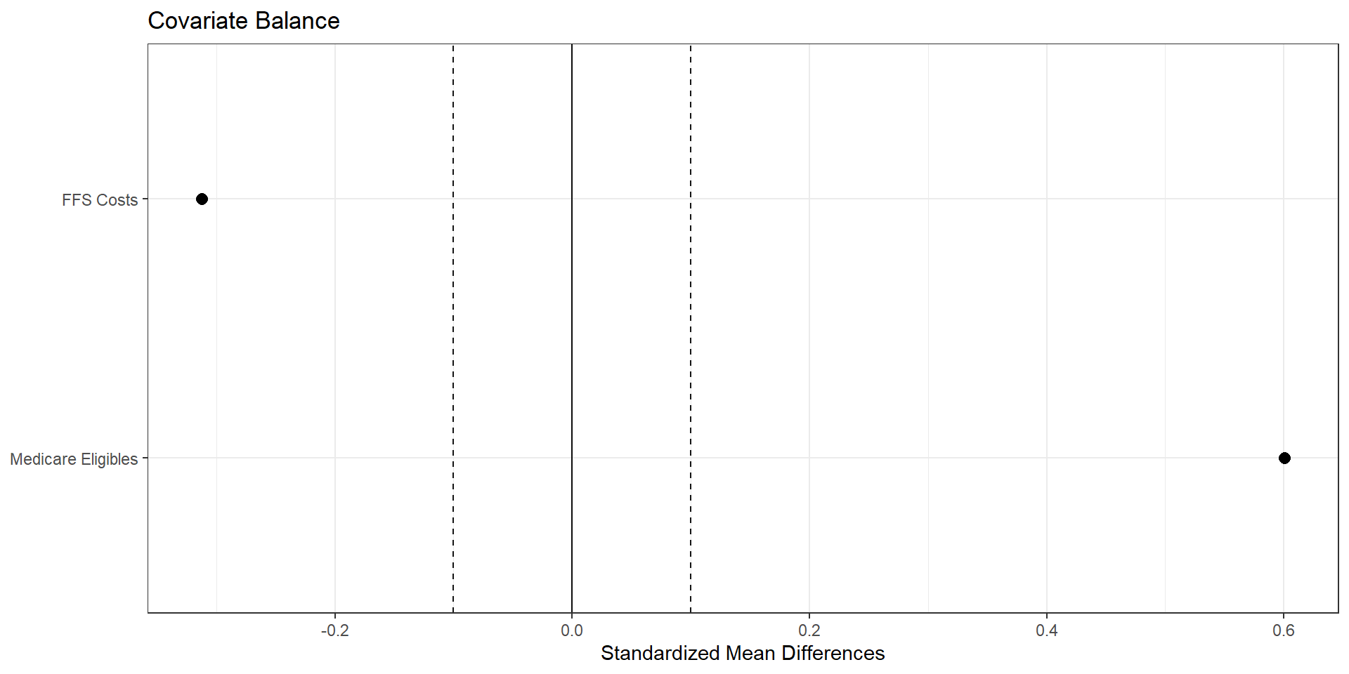
1. Exact Matching (on a subset)

lp.covs2 <- lp.covs %>% select(ffs_cost)
m.exact <- Matching::Match(Y=lp.vars$avg_bid,
                           Tr=lp.vars$treated_dummy,
                           X=lp.covs2,
                           M=1,
                           exact=TRUE,
                           estimand="ATE")

2. Nearest neighbor matching (inverse variance, many matches)

m.nn.var <- Matching::Match(Y=lp.vars$avg_bid,
                            Tr=lp.vars$treated_dummy,
                            X=lp.covs,
                            M=4,
                            Weight=1,
                            estimand="ATE")
import numpy as np
import pandas as pd
from sklearn.preprocessing import StandardScaler
from sklearn.neighbors import NearestNeighbors

# lp_df should contain:
#  - 'avg_bid' (outcome, like Y)
#  - 'treated_dummy' (0/1, like Tr)
#  - all columns in lp.covs (covariates for matching)

cov_cols = [
    "avg_eligibles",
    "ffs_cost",
]

# Drop missing
lp_df_cc = lp_df.dropna(subset=cov_cols + ["avg_bid", "treated_dummy"]).copy()

treated = lp_df_cc[lp_df_cc["treated_dummy"] == 1].copy()
controls = lp_df_cc[lp_df_cc["treated_dummy"] == 0].copy()

X_t = treated[cov_cols].values
X_c = controls[cov_cols].values
y_t = treated["avg_bid"].values
y_c = controls["avg_bid"].values

# Standardize covariates (rough analogue to Weight=1 / inverse-variance scaling)
scaler = StandardScaler()
X_c_scaled = scaler.fit_transform(X_c)
X_t_scaled = scaler.transform(X_t)

# Nearest neighbors: M = 4 matches per treated
M = 4
nn = NearestNeighbors(n_neighbors=M, metric="euclidean")
nn.fit(X_c_scaled)

distances, indices = nn.kneighbors(X_t_scaled, return_distance=True)

# For each treated unit, average its matched controls' outcomes
matched_ctrl_means = y_c[indices].mean(axis=1)

# ATT-style estimate: E[Y(1) - Y(0) | treated]
effect_nn = np.mean(y_t - matched_ctrl_means)

print("Nearest-neighbor estimate for avg_bid (treated - control):", effect_nn)


Estimate...  11.133 
AI SE......  3.7953 
T-stat.....  2.9333 
p.val......  0.003354 

Original number of observations..............  107 
Original number of treated obs...............  54 
Matched number of observations...............  107 
Matched number of observations  (unweighted).  428 

2. Nearest neighbor matching (inverse variance, one-to-one)

m.nn.var2 <- Matching::Match(Y=lp.vars$avg_bid,
                             Tr=lp.vars$treated_dummy,
                             X=lp.covs,
                             M=1,   #<<
                             Weight=1,
                             estimand="ATE")
import numpy as np
import pandas as pd
from sklearn.preprocessing import StandardScaler
from sklearn.neighbors import NearestNeighbors

# lp_df should contain:
#  - 'avg_bid' (outcome, like Y)
#  - 'treated_dummy' (0/1, like Tr)
#  - all columns in lp.covs (covariates for matching)

cov_cols = [
    "avg_eligibles",
    "ffs_cost",
]

# Drop missing
lp_df_cc = lp_df.dropna(subset=cov_cols + ["avg_bid", "treated_dummy"]).copy()

treated = lp_df_cc[lp_df_cc["treated_dummy"] == 1].copy()
controls = lp_df_cc[lp_df_cc["treated_dummy"] == 0].copy()

X_t = treated[cov_cols].values
X_c = controls[cov_cols].values
y_t = treated["avg_bid"].values
y_c = controls["avg_bid"].values

# Standardize covariates (rough analogue to Weight=1 / inverse-variance scaling)
scaler = StandardScaler()
X_c_scaled = scaler.fit_transform(X_c)
X_t_scaled = scaler.transform(X_t)

# Nearest neighbors: M = 1 match per treated
M = 1
nn = NearestNeighbors(n_neighbors=M, metric="euclidean")
nn.fit(X_c_scaled)

distances, indices = nn.kneighbors(X_t_scaled, return_distance=True)

# For each treated unit, average its matched controls' outcomes
matched_ctrl_means = y_c[indices].mean(axis=1)

# ATT-style estimate: E[Y(1) - Y(0) | treated]
effect_nn = np.mean(y_t - matched_ctrl_means)

print("Nearest-neighbor estimate for avg_bid (treated - control):", effect_nn)


Estimate...  11.726 
AI SE......  4.3248 
T-stat.....  2.7114 
p.val......  0.0067009 

Original number of observations..............  107 
Original number of treated obs...............  54 
Matched number of observations...............  107 
Matched number of observations  (unweighted).  107 

2. Nearest neighbor matching (Mahalanobis)

m.nn.md <- Matching::Match(Y=lp.vars$avg_bid,
                           Tr=lp.vars$treated_dummy,
                           X=lp.covs,
                           M=1,
                           Weight=2,
                           estimand="ATE")                           
import numpy as np
import pandas as pd
from sklearn.neighbors import NearestNeighbors

# Covariate set X (matching variables)
cov_cols = [
    "avg_eligibles",
    "ffs_cost",
]

# Drop missing on outcome / treatment / covariates
lp_df_cc = lp_df.dropna(subset=cov_cols + ["avg_bid", "treated_dummy"]).copy()

treated  = lp_df_cc[lp_df_cc["treated_dummy"] == 1].copy()
controls = lp_df_cc[lp_df_cc["treated_dummy"] == 0].copy()

X_t = treated[cov_cols].to_numpy()
X_c = controls[cov_cols].to_numpy()
y_t = treated["avg_bid"].to_numpy()
y_c = controls["avg_bid"].to_numpy()

# Pooled covariance of covariates (R's Matching uses Mahalanobis on X)
V = np.cov(np.vstack([X_t, X_c]).T)

# 1-nearest neighbor with Mahalanobis distance --------------------------
nn = NearestNeighbors(
    n_neighbors=1,
    metric="mahalanobis",
    metric_params={"V": V}
)
nn.fit(X_c)

distances, indices = nn.kneighbors(X_t, return_distance=True)

# Matched control outcomes
matched_ctrl = y_c[indices.flatten()]

# ATT-style effect (treated minus matched controls)
effect_nn_md = np.mean(y_t - matched_ctrl)

print("Mahalanobis 1-NN estimate for avg_bid (treated - control):", effect_nn_md)


Estimate...  11.416 
AI SE......  4.3543 
T-stat.....  2.6217 
p.val......  0.0087482 

Original number of observations..............  107 
Original number of treated obs...............  54 
Matched number of observations...............  107 
Matched number of observations  (unweighted).  107 

2. Nearest neighbor matching (propensity score)

logit.model <- glm(treated_dummy ~ avg_eligibles + ffs_cost, family=binomial, data=lp.vars)
ps <- fitted(logit.model)
m.nn.ps <- Matching::Match(Y=lp.vars$avg_bid,
                           Tr=lp.vars$treated_dummy,
                           X=ps,
                           M=1,
                           estimand="ATE")
import numpy as np
import pandas as pd
import statsmodels.formula.api as smf
from sklearn.neighbors import NearestNeighbors

# lp_df should contain:
#   - 'avg_bid'          (outcome)
#   - 'treated_dummy'    (0/1)
#   - 'avg_eligibles'
#   - 'ffs_cost'         # use 'ffs_cost' here if that's your column name

# 1. Estimate propensity scores ----------------------------------------
logit_res = smf.logit(
    "treated_dummy ~ avg_eligibles + ffs_cost",
    data=lp_df
).fit()

lp_df_ps = lp_df.copy()
lp_df_ps["ps"] = logit_res.predict(lp_df_ps)

# Optional: trim extreme PS
eps = 1e-6
lp_df_ps["ps"] = lp_df_ps["ps"].clip(eps, 1 - eps)

# 2. Prepare treated / control samples ---------------------------------
lp_df_cc = lp_df_ps.dropna(subset=["avg_bid", "treated_dummy", "ps"]).copy()

treated  = lp_df_cc[lp_df_cc["treated_dummy"] == 1].copy()
controls = lp_df_cc[lp_df_cc["treated_dummy"] == 0].copy()

y_t = treated["avg_bid"].to_numpy()
y_c = controls["avg_bid"].to_numpy()

X_t = treated[["ps"]].to_numpy()   # 1D propensity score as matching covariate
X_c = controls[["ps"]].to_numpy()

# 3. 1-nearest neighbor on propensity score (ATT-style) ----------------
nn = NearestNeighbors(n_neighbors=1, metric="euclidean")
nn.fit(X_c)

distances, indices = nn.kneighbors(X_t, return_distance=True)

matched_ctrl = y_c[indices.flatten()]

effect_ps_nn = np.mean(y_t - matched_ctrl)

print("PS 1-NN estimate for avg_bid (treated - control):", effect_ps_nn)
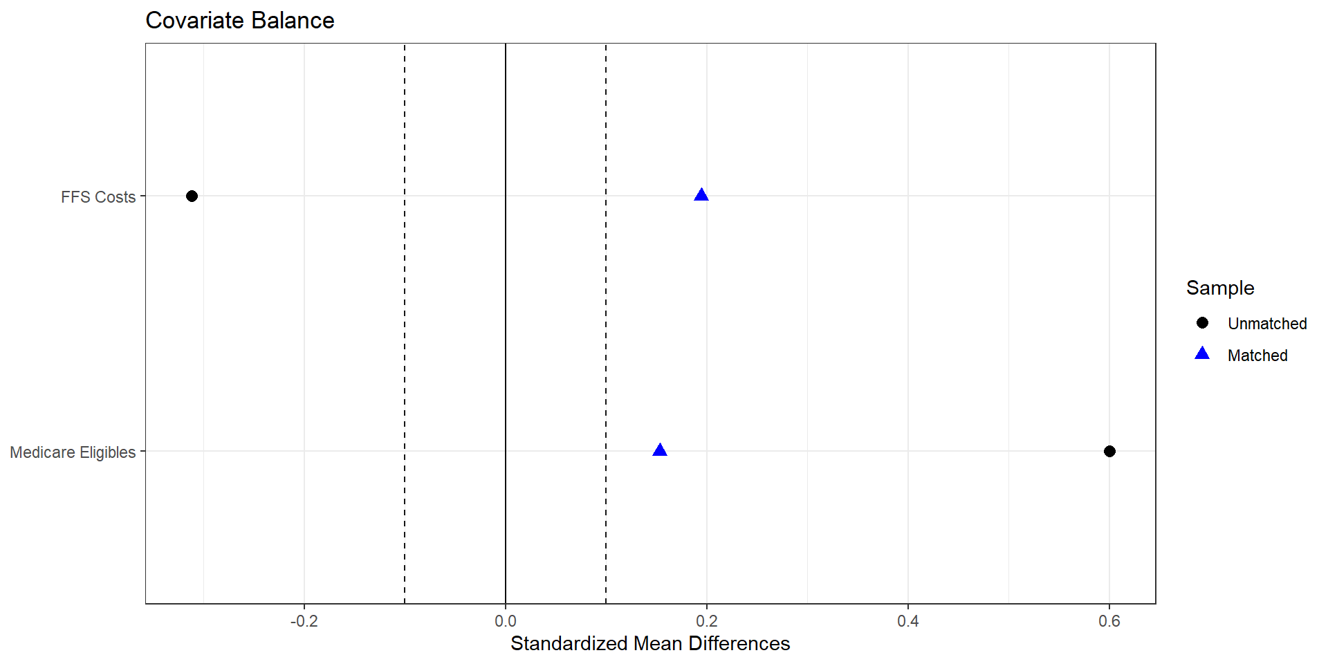

Estimate...  13.097 
AI SE......  4.6112 
T-stat.....  2.8402 
p.val......  0.0045081 

Original number of observations..............  107 
Original number of treated obs...............  54 
Matched number of observations...............  107 
Matched number of observations  (unweighted).  108 

3. Weighting with Simple Averages

lp.vars <- lp.vars %>%
  mutate(ipw = case_when(
    treated_dummy==1 ~ 1/ps,
    treated_dummy==0 ~ 1/(1-ps),
    TRUE ~ NA_real_
  ))
mean.t1 <- lp.vars %>% filter(treated_dummy==1) %>%
  select(avg_bid, ipw) %>% summarize(mean_bid=weighted.mean(avg_bid,w=ipw))
mean.t0 <- lp.vars %>% filter(treated_dummy==0) %>%
  select(avg_bid, ipw) %>% summarize(mean_bid=weighted.mean(avg_bid,w=ipw))
import numpy as np
import pandas as pd

p_vars = lp_df.copy()

# Inverse probability weights
p_vars["ipw"] = np.where(
    p_vars["treated_dummy"] == 1,
    1.0 / p_vars["ps"],
    1.0 / (1.0 - p_vars["ps"])
)

# Treated group weighted mean of avg_bid
treated = p_vars[p_vars["treated_dummy"] == 1]
mean_t1 = np.average(treated["avg_bid"], weights=treated["ipw"])

# Control group weighted mean of avg_bid
controls = p_vars[p_vars["treated_dummy"] == 0]
mean_t0 = np.average(controls["avg_bid"], weights=controls["ipw"])

ate_ipw = mean_t1 - mean_t0
print("IPW mean (treated):", mean_t1)
print("IPW mean (control):", mean_t0)
print("IPW ATE (treated - control):", ate_ipw)
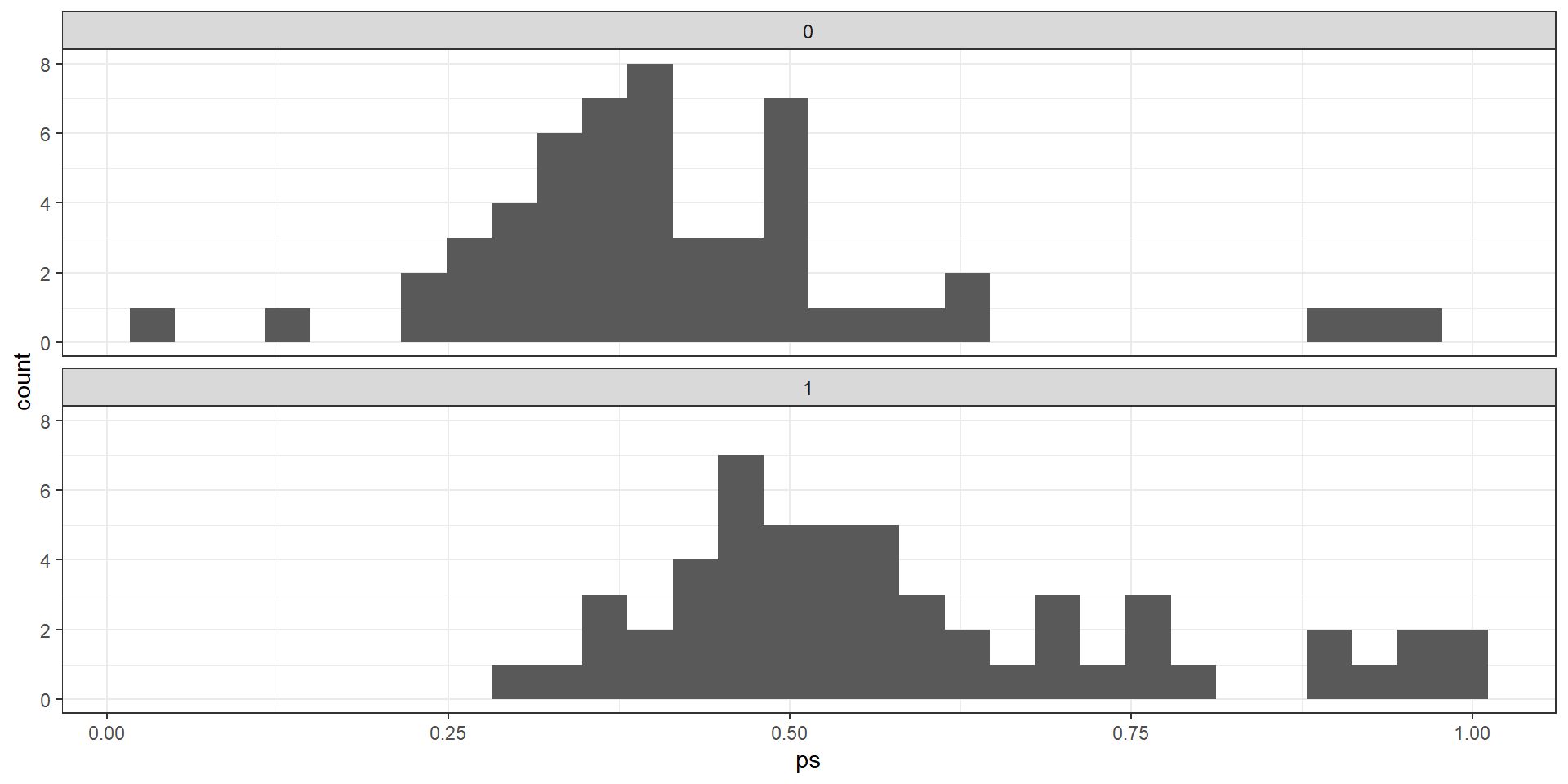
[1] 6.301051

3. Weighting with Regression

ipw.reg <- lm(avg_bid ~ treated_dummy, data=lp.vars, weights=ipw)
import statsmodels.formula.api as smf

# Assume lp_df has columns: avg_bid, treated_dummy, ipw
ipw_mod = smf.wls("avg_bid ~ treated_dummy",
                  data=lp_df,
                  weights=lp_df["ipw"]).fit()

print(ipw_mod.summary())
ate_ipw = ipw_mod.params["treated_dummy"]
summary(ipw.reg)

Call:
lm(formula = avg_bid ~ treated_dummy, data = lp.vars, weights = ipw)

Weighted Residuals:
    Min      1Q  Median      3Q     Max 
-77.344 -23.517  -3.087  13.099 100.832 

Coefficients:
              Estimate Std. Error t value Pr(>|t|)    
(Intercept)    864.166      2.644 326.835   <2e-16 ***
treated_dummy    6.301      4.055   1.554    0.123    
---
Signif. codes:  0 '***' 0.001 '**' 0.01 '*' 0.05 '.' 0.1 ' ' 1

Residual standard error: 30.81 on 105 degrees of freedom
Multiple R-squared:  0.02248,   Adjusted R-squared:  0.01317 
F-statistic: 2.415 on 1 and 105 DF,  p-value: 0.1232

4. Regression without Weighting

# Two-step regression
reg1.dat <- lp.vars %>% filter(treated_dummy==1, complete.cases(.))
reg1 <- lm(avg_bid ~ ffs_cost + avg_eligibles, data=reg1.dat)

reg0.dat <- lp.vars %>% filter(treated_dummy==0, complete.cases(.))
reg0 <- lm(avg_bid ~ ffs_cost + avg_eligibles, data=reg0.dat)
pred1 <- predict(reg1,new=lp.vars)
pred0 <- predict(reg0,new=lp.vars)

# One-step regression
reg.dat <- lp.vars %>% ungroup() %>% filter(complete.cases(.)) %>%
  mutate(ffs_diff = treated_dummy*(ffs_cost - mean(ffs_cost)),
         eligibles_diff = treated_dummy*(avg_eligibles - mean(avg_eligibles)))
reg <- lm(avg_bid ~ treated_dummy + ffs_cost + avg_eligibles +
            ffs_diff + eligibles_diff,
          data=reg.dat)
import pandas as pd
import statsmodels.formula.api as smf

# lp_df is the Python analogue of lp.vars
# It must contain: avg_bid, treated_dummy, ffs_cost, avg_eligibles

# ---------------------------------------------------------
# 1. Two separate regressions by treatment, then predict
# ---------------------------------------------------------

# Complete cases for the variables we need
cols_needed = ["avg_bid", "treated_dummy", "ffs_cost", "avg_eligibles"]
lp_complete = lp_df.dropna(subset=cols_needed).copy()

# Treated: treated_dummy == 1
reg1_data = lp_complete[lp_complete["treated_dummy"] == 1]
reg1 = smf.ols("avg_bid ~ ffs_cost + avg_eligibles", data=reg1_data).fit()

# Controls: treated_dummy == 0
reg0_data = lp_complete[lp_complete["treated_dummy"] == 0]
reg0 = smf.ols("avg_bid ~ ffs_cost + avg_eligibles", data=reg0_data).fit()

# Predict avg_bid for everyone under each regime
pred1 = reg1.predict(lp_df)  # E[avg_bid | treated=1, X]
pred0 = reg0.predict(lp_df)  # E[avg_bid | treated=0, X]

# ---------------------------------------------------------
# 2. One-step regression with interactions
# ---------------------------------------------------------

reg_df = lp_complete.copy()  # already complete on needed cols

ffs_mean   = reg_df["ffs_cost"].mean()
elig_mean  = reg_df["avg_eligibles"].mean()

reg_df["ffs_diff"]        = reg_df["treated_dummy"] * (reg_df["ffs_cost"] - ffs_mean)
reg_df["eligibles_diff"]  = reg_df["treated_dummy"] * (reg_df["avg_eligibles"] - elig_mean)

reg = smf.ols(
    "avg_bid ~ treated_dummy + ffs_cost + avg_eligibles + ffs_diff + eligibles_diff",
    data=reg_df
).fit()

print(reg.summary())
[1] 12.56089

Call:
lm(formula = avg_bid ~ treated_dummy + ffs_cost + avg_eligibles + 
    ffs_diff + eligibles_diff, data = reg.dat)

Residuals:
    Min      1Q  Median      3Q     Max 
-47.121 -11.398   0.933  12.368  41.839 

Coefficients:
                 Estimate Std. Error t value Pr(>|t|)    
(Intercept)     8.433e+02  1.793e+01  47.043  < 2e-16 ***
treated_dummy   1.256e+01  3.910e+00   3.212 0.001768 ** 
ffs_cost        2.605e-04  1.670e-03   0.156 0.876325    
avg_eligibles   1.385e-03  3.565e-04   3.884 0.000183 ***
ffs_diff        3.374e-03  3.838e-03   0.879 0.381411    
eligibles_diff -1.178e-03  3.841e-04  -3.067 0.002776 ** 
---
Signif. codes:  0 '***' 0.001 '**' 0.01 '*' 0.05 '.' 0.1 ' ' 1

Residual standard error: 18.2 on 101 degrees of freedom
Multiple R-squared:  0.3104,    Adjusted R-squared:  0.2763 
F-statistic: 9.094 on 5 and 101 DF,  p-value: 3.64e-07

Summary of ATEs

  1. Exact matching: no matches available
  2. NN matching, inverse variance: 11.73
  3. NN matching, mahalanobis: 11.42
  4. NN matching, pscore: 13.1
  5. IPW weighting: 6.3
  6. IPW regression: 6.3
  7. Regression 2-step: 12.56
  8. Regression 1-step: 12.56

Summary of ATEs

Why such large differences between IPW and other approaches?

Problem is due to common support in the propensity scores. Failure to account for this severly deflates estimates.

Adjusting for poor overlap

R Code
mean.t1 <- lp.vars %>% filter(treated_dummy==1, ps>0.15, ps<0.95) %>%
  select(avg_bid, ipw) %>% summarize(mean_bid=weighted.mean(avg_bid,w=ipw))
mean.t0 <- lp.vars %>% filter(treated_dummy==0, ps>0.15, ps<0.95) %>%
  select(avg_bid, ipw) %>% summarize(mean_bid=weighted.mean(avg_bid,w=ipw))
print(mean.t1-mean.t0)
  mean_bid
1 10.08417

So what have we learned?

Key assumptions for causal inference so far

  1. Selection on observables
  2. Common support

Causal effect assuming selection on observables

If we assume selection on observables holds, then we only need to condition on the relevant covariates to identify a causal effect. But we still need to ensure common support.

  1. Matching
  2. Reweighting
  3. Regression