More Medicare Advantage Data

Ian McCarthy | Emory University

Outline for Today

  1. Revisit Medicare Advantage Data
  2. Examine Relationship between Ratings and Enrollments

Medicare Advantage Data

Building the Data

Recall from the last two homework assignments (or snippets of those data, focusing on GA in 2022)

  • ga_plans_year – yearly GA plan panel (from contracts + enrollment).
  • ga_service_year – yearly GA service-area panel.
  • ga_landscape – GA plan characteristics (landscape, incl. premium_partc).
  • ga_penetration – GA penetration data.
  • Now incorporate yearly star-ratings files

Understanding the Ratings Data

  • Underlying measures change from year to year
  • File rating_variables.R lists the relevant variables for each year
  • partc_score reflects specific star rating for Part C
    • Compilation of all underying measures plus additional adjustments
    • For our purposes…just use the average of the underying measures

Contracts versus Plans

  • Recall the difference between contractid and planid
  • Star ratings are calculated at the contract level
    • Applies to all plans operating under the same contractid
    • Applies to all counties in which the same contractid is approved
  • For our purposes…treat everything at the plan level

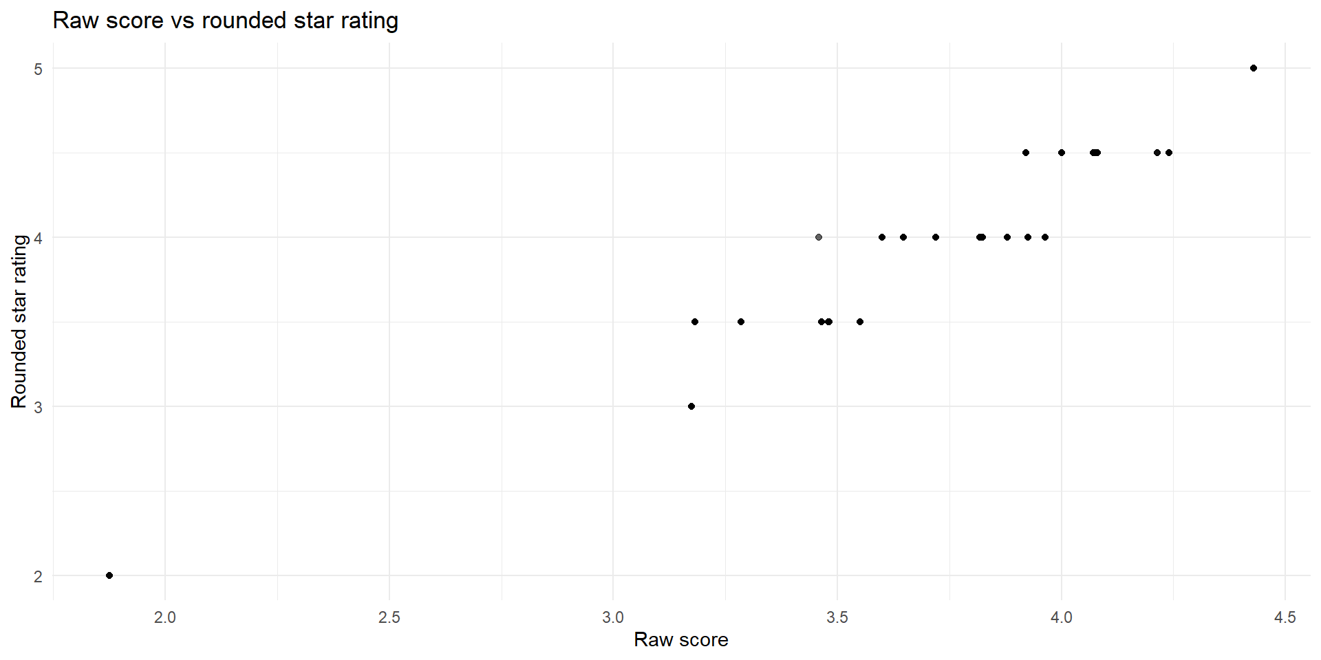
Example: Star Ratings in 2022

ga_ma_2022 <- read_csv("../data/output/ma-snippets/ga-ma-data-2022.csv") %>%
  select(-partc_score) %>% ungroup()

ma_ratings <- read_csv("../data/output/ma-snippets/ga-ratings-2022.csv")

ga_ma_full <- ga_ma_2022 %>%
  left_join(ma_ratings, by="contractid") %>%
  mutate(raw_rating=rowMeans(
    cbind(breastcancer_screen, rectalcancer_screen, flu_vaccine,
          physical_monitor, specialneeds_manage, older_medication, older_pain,
          osteo_manage, diabetes_eye, diabetes_kidney, diabetes_bloodsugar,
          ra_manage, falling, bladder, medication, statin, nodelays,
          carequickly, customer_service, overallrating_care, overallrating_plan,
          coordination, complaints_plan, leave_plan, improve, appeals_timely,
          appeals_review, ttyt_available),
    na.rm=T)) %>%
    select(contractid, planid, fips, plan_type, partd, avg_enrollment, avg_eligibles,
           avg_enrolled, premium, premium_partc, premium_partd, rebate_partc, ma_rate,
           bid, avg_ffscost, partc_score, partcd_score, raw_rating)
import pandas as pd

# Read in data
ga_ma_2022 = (
    pd.read_csv("../data/output/ma-snippets/ga-ma-data-2022.csv")
    .drop(columns=["partc_score"], errors="ignore")
)

ma_ratings = pd.read_csv("../data/output/ma-snippets/ga-ratings-2022.csv")

# Merge on contractid
ga_ma_full = ga_ma_2022.merge(ma_ratings, on="contractid", how="left")

# Variables used to construct the raw rating
rating_vars = [
    "breastcancer_screen", "rectalcancer_screen", "flu_vaccine",
    "physical_monitor", "specialneeds_manage", "older_medication", "older_pain",
    "osteo_manage", "diabetes_eye", "diabetes_kidney", "diabetes_bloodsugar",
    "ra_manage", "falling", "bladder", "medication", "statin", "nodelays",
    "carequickly", "customer_service", "overallrating_care", "overallrating_plan",
    "coordination", "complaints_plan", "leave_plan", "improve", "appeals_timely",
    "appeals_review", "ttyt_available"
]

# Row-wise mean, ignoring missing values (na.rm = TRUE)
ga_ma_full["raw_rating"] = ga_ma_full[rating_vars].mean(axis=1, skipna=True)

# Keep the desired columns
ga_ma_full = ga_ma_full[
    [
        "contractid", "planid", "fips", "plan_type", "partd", "avg_enrollment",
        "avg_eligibles", "avg_enrolled", "premium", "premium_partc",
        "premium_partd", "rebate_partc", "ma_rate", "bid", "avg_ffscost",
        "partc_score", "partcd_score", "raw_rating"
    ]
]

R Code
rounding_counts_3_75 <- ga_ma_full %>%
  filter(
    !is.na(raw_rating), !is.na(partc_score),
    partc_score %in% c(3.5, 4.0),
    raw_rating >= 3.5, raw_rating <= 4.0, 
    (raw_rating >= 3.75 & partc_score==4.0) | (raw_rating <= 3.75 & partc_score==3.5)
  ) %>%
  mutate(
    `Raw Score` = if_else(raw_rating >= 3.75, "≥ 3.75", "< 3.75"),
    `Star`   = if_else(partc_score == 4.0, "4.0", "3.5")
  ) %>%
  count(`Raw Score`, `Star`, name = "Plans")

rounding_counts_3_75 %>%
  kbl(
    format  = "html",
    caption = "Ratings vs Raw Score"
  ) %>%
  kable_styling(
    bootstrap_options = c("striped", "hover", "condensed"),
    full_width        = FALSE,
    position          = "center"
  )
Ratings vs Raw Score
Raw Score Star Plans
< 3.75 3.5 35
≥ 3.75 4.0 359

Enrollments and Star Ratings

Summary stats

Focus on enrollments and star ratings:

miss_n <- function(x) sum(is.na(x))
sum.vars <- ga_ma_full %>% 
      select("MA Enrollment" = avg_enrollment, "MA Eligibles" = avg_eligibles, "Star Rating" = partc_score,
             "Raw Score" = raw_rating)
datasummary(All(sum.vars) ~ Mean + SD + miss_n + Histogram, data=sum.vars, fmt=2)
Mean SD miss_n Histogram
MA Enrollment 153.62 456.49 0.00
MA Eligibles 19141.94 28803.30 0.00 ▇▂▁
Star Rating 3.97 0.52 3.00 ▁▆▃▇
Raw Score 3.74 0.34 0.00 ▂▄▁▇
import pandas as pd
import numpy as np

# 1. Subset and rename variables (analogous to select + renaming in R)
sum_vars = ga_ma_full.rename(columns={
    "avg_enrollment": "MA Enrollment",
    "avg_eligibles":  "MA Eligibles",
    "partc_score":    "Star Rating",
    "raw_rating":     "Raw Score",
})[["MA Enrollment", "MA Eligibles", "Star Rating", "Raw Score"]]

# 2. Define missing-count function (miss_n)
def miss_n(x):
    return x.isna().sum()

# 3. (Optional) simple text histogram for each variable
def hist_text(x, bins=10):
    counts, _ = np.histogram(x.dropna(), bins=bins)
    return " | ".join(map(str, counts))

# 4. Build summary table: Mean, SD, missing, and histogram
summary = pd.DataFrame({
    "Mean":      sum_vars.mean(),
    "SD":        sum_vars.std(),
    "Missing N": sum_vars.apply(miss_n),
    "Histogram": sum_vars.apply(hist_text),  # drop this line if you don't want the histogram column
})

# 5. Optional: format to 2 decimal places for Mean and SD
summary[["Mean", "SD"]] = summary[["Mean", "SD"]].round(2)

summary

Simple regression

rating.ols <- lm(avg_enrollment~factor(partc_score), data=ga_ma_full)
import statsmodels.formula.api as smf

rating_ols = smf.ols("avg_enrollment ~ C(partc_score)", data=ga_ma_full).fit()
print(rating_ols.summary())

Call:
lm(formula = avg_enrollment ~ factor(partc_score), data = ga_ma_full)

Residuals:
   Min     1Q Median     3Q    Max 
-716.7 -134.4  -98.1  -30.6 9728.5 

Coefficients:
                       Estimate Std. Error t value Pr(>|t|)   
(Intercept)               13.07     225.54   0.058  0.95378   
factor(partc_score)3      40.11     227.50   0.176  0.86005   
factor(partc_score)3.5   106.60     225.96   0.472  0.63713   
factor(partc_score)4     187.91     226.26   0.831  0.40631   
factor(partc_score)4.5   147.81     225.89   0.654  0.51294   
factor(partc_score)5     715.46     237.12   3.017  0.00257 **
---
Signif. codes:  0 '***' 0.001 '**' 0.01 '*' 0.05 '.' 0.1 ' ' 1

Residual standard error: 451.1 on 3275 degrees of freedom
  (3 observations deleted due to missingness)
Multiple R-squared:  0.02584,   Adjusted R-squared:  0.02436 
F-statistic: 17.38 on 5 and 3275 DF,  p-value: < 2.2e-16

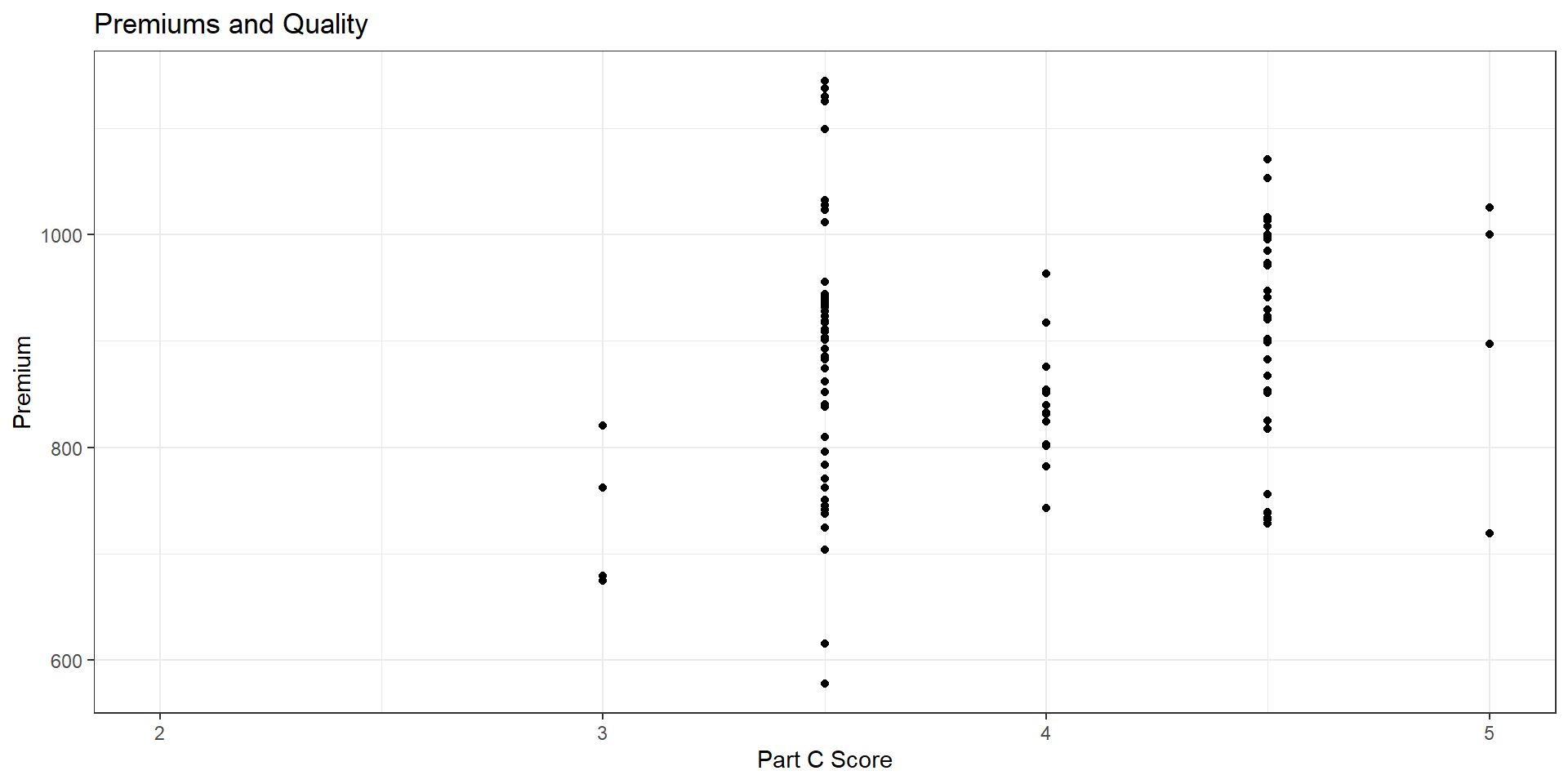
Potential endogeneity

  • The star rating is a measure of quality
  • Actual “quality” is not the same as “quality disclosure”
  • Quality may be endogenous to enrollment (how?)


Call:
lm(formula = bid ~ factor(partc_score), data = ga_ma_full)

Residuals:
     Min       1Q   Median       3Q      Max 
-261.079  -71.049    9.059   70.648  305.049 

Coefficients:
                       Estimate Std. Error t value Pr(>|t|)    
(Intercept)             750.240      6.714 111.739  < 2e-16 ***
factor(partc_score)3.5   89.295      7.392  12.079  < 2e-16 ***
factor(partc_score)4     80.448      7.853  10.244  < 2e-16 ***
factor(partc_score)4.5  181.633      7.284  24.936  < 2e-16 ***
factor(partc_score)5    119.729     17.831   6.715 2.21e-11 ***
---
Signif. codes:  0 '***' 0.001 '**' 0.01 '*' 0.05 '.' 0.1 ' ' 1

Residual standard error: 101.8 on 3272 degrees of freedom
  (7 observations deleted due to missingness)
Multiple R-squared:  0.2319,    Adjusted R-squared:  0.2309 
F-statistic: 246.9 on 4 and 3272 DF,  p-value: < 2.2e-16