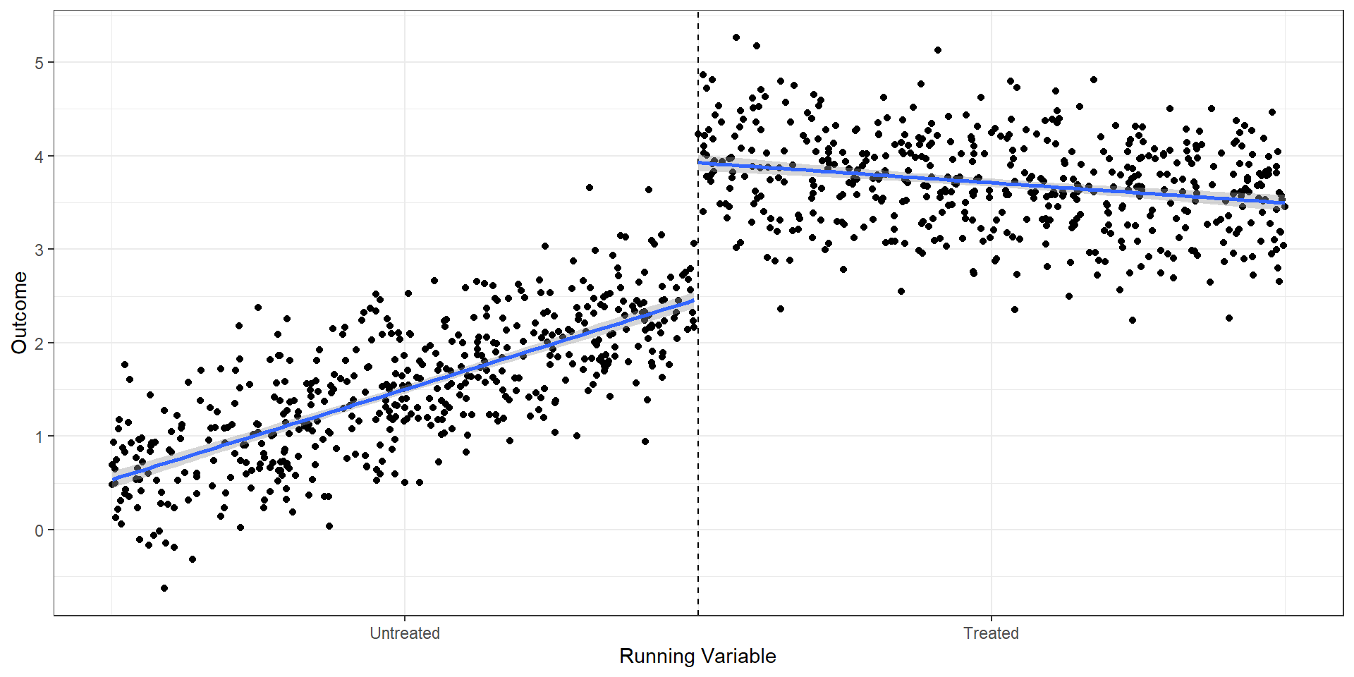
Now the slope can differ above and below the cutoff
\(\gamma\) captures the difference in slopes
More flexible, but uses more degrees of freedom in small bandwidths
Beyond linear
Can add polynomials in \(\tilde{X}\) and interactions with \(D\)
In practice, local linear (the previous two slides) is the standard
Higher-order polynomials are generally discouraged (more on this later)
Key RD Steps
Show clear graphical evidence of a change around the discontinuity (bin scatter)
Balance above/below threshold (use baseline covariates as outcomes)
Manipulation tests
RD estimates
Sensitivity and robustness:
Bandwidths
Order of polynomial
Inclusion of covariates
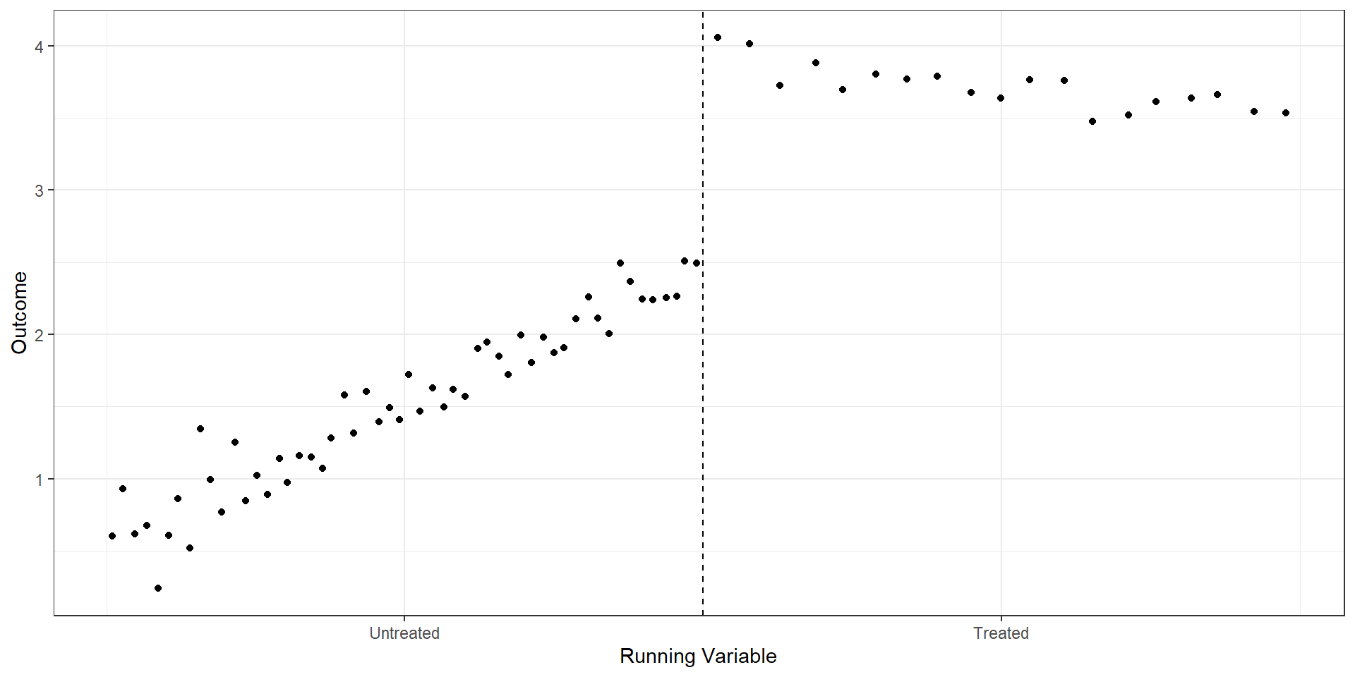
1. Graphical evidence
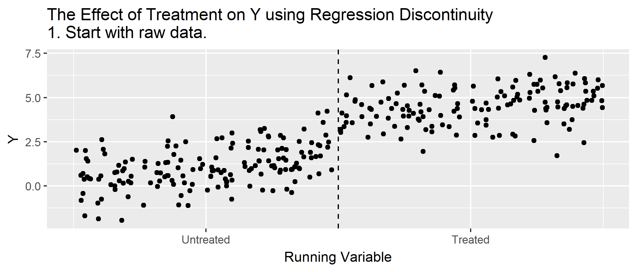
Before presenting RD estimates, any good RD approach first highlights the discontinuity with a simple graph. We can do so by plotting the average outcomes within bins of the forcing variable (i.e., binned averages), \[\bar{Y}_{k} = \frac{1}{N_{k}}\sum_{i=1}^{N} Y_{i} \times 1(b_{k} < X_{i} \leq b_{k+1}).\]
The binned averages helps to remove noise in the graph and can provide a cleaner look at the data. Just make sure that no bin includes observations above and below the cutoff!
import pandas as pdimport seaborn as snsimport matplotlib.pyplot as pltfrom rdrobust import rdplot# rd_dat is a pandas DataFrame with columns "Y" and "X"# Run rdplot but suppress its own figure and grab the binned datard_result = rdplot( y=rd_dat["Y"].values, x=rd_dat["X"].values, c=1, title="RD Plot with Binned Average", x_label="Running Variable", y_label="Outcome", hide=True# don't show the built-in plot)# vars_bins is already a pandas DataFrame in the Python implementationbin_avg = rd_result.vars_bins# Recreate the custom plotsns.set_style("whitegrid")fig, ax = plt.subplots()sns.scatterplot( data=bin_avg, x="rdplot_mean_x", y="rdplot_mean_y", ax=ax)ax.axvline(x=1, linestyle="--", color="black")ax.set_xticks([0.5, 1.5])ax.set_xticklabels(["Untreated", "Treated"])ax.set_xlabel("Running Variable")ax.set_ylabel("Outcome")ax.set_title("RD Plot with Binned Average")sns.despine()plt.tight_layout()plt.show()
Selecting “bin” width
How many bins should we use? Too few and we obscure the discontinuity; too many and the graph is noisy.
Bin width: formal tests
Dummy variable approach: Create dummies for each bin, regress outcome on the dummies (\(R^{2}_{r}\)). Double the number of bins (\(R^{2}_{u}\)). F-test: \[F = \frac{R^{2}_{u}-R^{2}_{r}}{1-R^{2}_{u}}\times \frac{n-K-1}{K}\]
Interaction approach: Include interactions between bin dummies and the running variable, then joint F-test on the interaction terms
If significant, we have too few bins and should narrow the width.
2. Balance
If RD is an appropriate design, passing the cutoff should only affect treatment and outcome of interest
How do we test for this?
Covariate balance
Placebo tests of other outcomes (e.g., t-1 outcomes against treatment at time t)
3. Manipulation tests
Individuals should not be able to precisely manipulate running variable to enter into treatment
Sometimes discussed as “bunching”
Test for differences in density to left and right of cutoffs (rddensity)
Permutation tests proposed in Ganong and Jager (2017)
What if there is bunching?
Gerard, Rokkanen, and Rothe (2020) suggest partial identification allowing for bunching
Can also be used as a robustness check (rdbounds)
Assumption: bunching only moves people in one direction
4. RD Estimation
Start with the “default” options
Local linear regression
Optimal bandwidth
Uniform kernel
Selecting bandwidth
The bandwidth is a “tuning parameter”
High \(h\) means high bias but lower variance (use more of the data, closer to OLS)
Low \(h\) means low bias but higher variance (use less data, more focused around discontinuity)
Represent bias-variance tradeoff with the mean-square error, \[MSE(h) = E[(\hat{\tau}_{h} - \tau_{RD})^2]=\left(E[\hat{\tau}_{h} - \tau_{RD}] \right)^2 + V(\hat{\tau}_{h}).\]
Selecting bandwidth
In the RD case, we have two different mean-square error terms:
Goal is to find \(h\) that minimizes these values, but we don’t know the true \(E[Y_{1}|X=c]\) and \(E[Y_{0}|X=c]\). So we have two approaches:
Use cross-validation to choose \(h\)
Explicitly solve for optimal bandwidth
Cross-validation
Essentially a series of “leave-one-out” estimates:
Pick an \(h\)
Run regression, leaving out observation \(i\). If \(i\) is to the left of the threshold, we estimate regression for observations within \(X_{i}-h\), and conversely \(X_{i}+h\) if \(i\) is to the right of the threshold.
Predicted \(\hat{Y}_{i}\) at \(X_{i}\) (out of sample prediction for the left out observation)
Do this for all \(i\), and form \(CV(h)=\frac{1}{N}\sum (Y_{i} - \hat{Y}_{i})^2\)
import pandas as pdimport statsmodels.formula.api as smf# OLS on full sampleols = smf.ols("Y ~ X + W", data=rd_dat).fit()# Local linear regression around cutoff X = 1rd_dat3 = ( rd_dat .assign(x_dev=lambda df: df["X"] -1) .query("X > 0.8 and X < 1.2"))rd = smf.ols("Y ~ x_dev + W", data=rd_dat3).fit()
from rdrobust import rdrobust# rd_dat is a pandas DataFrame with columns "Y" and "X"rd_y = rd_dat["Y"].valuesrd_x = rd_dat["X"].valuesrd_est = rdrobust(y=rd_y, x=rd_x, c=1)# Print a summary (rdrobust returns a custom object with its own __str__)print(rd_est)
Sharp RD estimates using local polynomial regression.

Number of Obs.                 1000
BW type                       mserd
Kernel                   Triangular
VCE method                       NN

Number of Obs.                  490          510
Eff. Number of Obs.             152          166
Order est. (p)                    1            1
Order bias  (q)                   2            2
BW est. (h)                   0.320        0.320
BW bias (b)                   0.497        0.497
rho (h/b)                     0.644        0.644
Unique Obs.                     490          510

=====================================================================
                   Point    Robust Inference
                Estimate         z     P>|z|      [ 95% C.I. ]
---------------------------------------------------------------------
     RD Effect     1.739    12.381     0.000     [1.475 , 2.030]
=====================================================================
Cattaneo et al. (2020) argue:
Report conventional point estimate
Report robust confidence interval
5. Robustness and sensitivity
Results should be stable across reasonable specification choices:
Bandwidths: try half and double the optimal bandwidth. If the estimate swings wildly, the result is fragile.
Kernels: uniform (equal weight) vs. triangular (more weight near cutoff). Should tell similar stories.
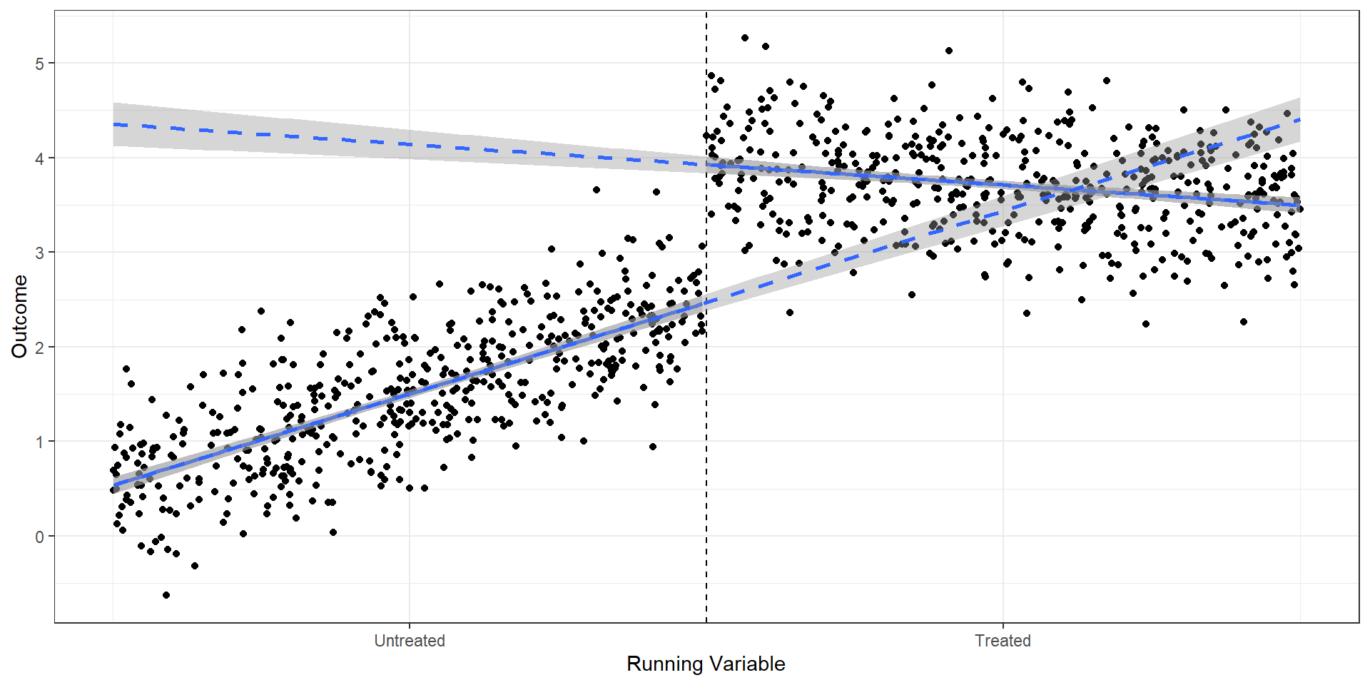
Polynomials: linear vs. quadratic. If you need a cubic to find the effect, worry.
Covariates: adding pre-treatment controls shouldn’t change the estimate much (they should be balanced at the cutoff). But they can improve precision.
Pitfalls of polynomials
Assign too much weight to points away from the cutoff
Results highly sensitive to degree of polynomial
Narrow confidence intervals (over-rejection of the null)
“Fuzzy” just means that assignment isn’t guaranteed based on the running variable. For example, maybe students are much more likely to get a scholarship past some threshold SAT score, but it remains possible for students below the threshold to still get the scholarship.
Discontinuity reflects a jump in the probability of treatment
Other RD assumptions still required (namely, can’t manipulate running variable around the threshold)
Fuzzy RD is IV
In practice, fuzzy RD is employed as an instrumental variables estimator
Difference in outcomes among those above and below the discontinuity divided by the difference in treatment probabilities for those above and below the discontinuity, \[E[Y_{i} | D_{i}=1] - E[Y_{i} | D_{i}=0] = \frac{E[Y_{i} | x_{i}\geq c] - E[Y_{i} | x_{i}< c]}{E[D_{i} | x_{i}\geq c] - E[D_{i} | x_{i}<c]}\]
Indicator for \(x_{i}\geq c\) is an instrument for treatment status, \(D_{i}\).