Regression Discontinuity: Part II
Binned Scatterplot
rd.result <- rdplot(ma_25star$mkt_share, ma_25star$raw_rating,
                    c=2.25, p=2,
                    title="RD Plot with Binned Average",
                    x.label="Running Variable",
                    y.label="Outcome",
                    hide = TRUE)
bin.avg <- as_tibble(rd.result$vars_bins)
plot.bin <- bin.avg %>% ggplot(aes(x=rdplot_mean_x,y=rdplot_mean_y)) +
  geom_point() + theme_bw() +
  geom_vline(aes(xintercept=2.25),linetype='dashed') +
  scale_x_continuous(
    breaks = c(2, 2.125, 2.25, 2.375, 2.5),
    label = c("2.0", "2.125", "2.25", "2.375", "2.5")
  ) +
  xlab("Raw Rating") + ylab("Market Share") +
  annotate("text", x=2.25, y=Inf, label="2.5-star\ncutoff",
           vjust=1.5, hjust=-0.1, size=3.5, color="grey40")
import pandas as pd
import matplotlib.pyplot as plt
from rdrobust import rdplot
# RD plot using mkt_share as outcome and raw_rating as running variable
rd_result = rdplot(
y=ma_25star["mkt_share"].values,
x=ma_25star["raw_rating"].values,
c=2.25,
title="RD Plot with Binned Average",
x_label="Running Variable",
y_label="Outcome",
hide=True # don't show the built-in plot
)
# vars_bins is already a pandas DataFrame in the Python implementation
bin_avg = rd_result.vars_bins
# Recreate the custom plot
fig, ax = plt.subplots()
ax.scatter(
bin_avg["rdplot_mean_x"],
bin_avg["rdplot_mean_y"]
)
ax.axvline(x=2.25, linestyle="--", color="grey")
ax.set_xticks([2.0, 2.125, 2.25, 2.375, 2.5])
ax.set_xticklabels(["2.0", "2.125", "2.25", "2.375", "2.5"])
ax.set_xlabel("Raw Rating")
ax.set_ylabel("Market Share")
ax.set_title("RD Plot with Binned Average")
ax.annotate("2.5-star\ncutoff", xy=(2.25, ax.get_ylim()[1]),
xytext=(2.27, ax.get_ylim()[1]*0.95), fontsize=9, color="grey")
plt.tight_layout()
plt.show()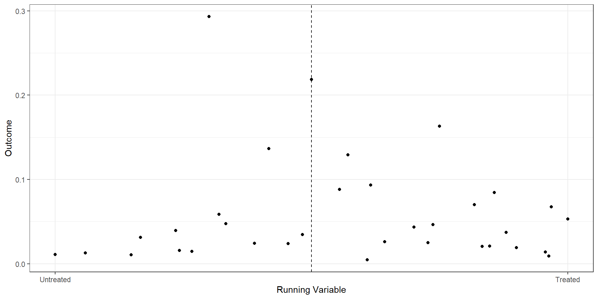
Manipulation of the running variable
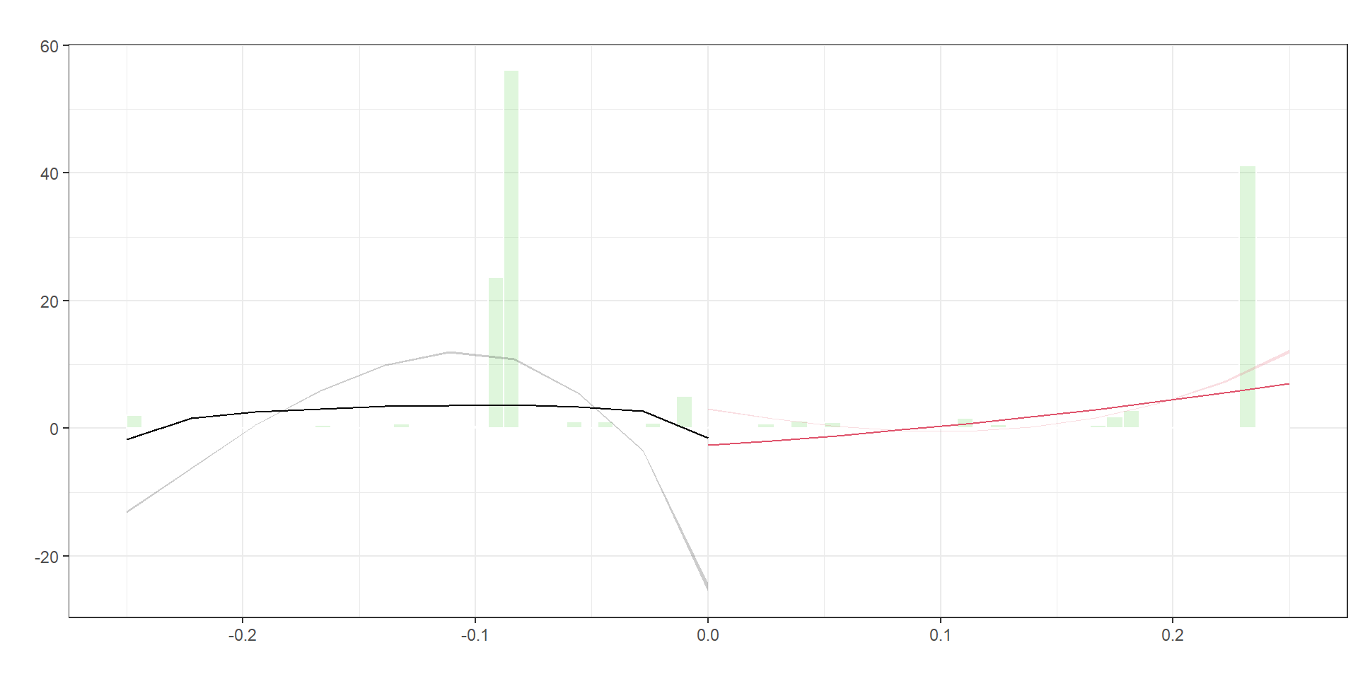
from rdrobust import rddensity, rdplotdensity
import matplotlib.pyplot as plt

# Run McCrary-style density test at cutoff 0
dens1 = rddensity(x=ma_rd1["score"].values, c=0)

# Create the density plot object (rdplotdensity returns a matplotlib figure/axes)
densplot = rdplotdensity(dens1, x=ma_rd1["score"].values)

# If you want to explicitly show or tweak:
fig = densplot["fig"]
ax = densplot["ax"]

ax.set_title("Density test around cutoff")
ax.set_xlabel("Score")
ax.set_ylabel("Estimated density")

plt.show()| Value | |
|---|---|
| T-statistic | 55.91 |
| P-value | 0.00 |
Interpretation: A large p-value means we cannot reject equal density on both sides of the cutoff, which is what we want. No evidence of manipulation.
Covariate balance
import numpy as np
import pandas as pd
from sklearn.neighbors import NearestNeighbors
import matplotlib.pyplot as plt

# 1. Subset data as in your R code
sub = (
    ma_rd1
    .loc[
        (ma_rd1["window2"]) &
        ma_rd1["treat"].notna() &
        ma_rd1["premium_partc"].notna() &
        ma_rd1["ma_rate"].notna()
    ]
    .copy()
)

covariates = ["premium_partc", "ma_rate"]

X = sub[covariates].to_numpy()
t = sub["treat"].astype(int).to_numpy()

# 2. Mahalanobis nearest-neighbor matching (1:1)
#    Estimate covariance matrix of covariates and its inverse
V = np.cov(X, rowvar=False)
V_inv = np.linalg.inv(V)

# Fit NN on controls only
nn = NearestNeighbors(
    n_neighbors=1,
    metric="mahalanobis",
    metric_params={"V": V}
)
nn.fit(X[t == 0])

# For each treated unit, find nearest control
dist, idx = nn.kneighbors(X[t == 1])
control_matches = sub.loc[t == 0].iloc[idx[:, 0]].copy()
treated_matched = sub.loc[t == 1].copy()

# Build matched sample
matched = pd.concat(
    [
        treated_matched.reset_index(drop=True),
        control_matches.reset_index(drop=True)
    ],
    axis=0
).reset_index(drop=True)
matched["treat"] = np.r_[np.ones(len(treated_matched)), np.zeros(len(control_matches))]

# 3. Function for standardized mean differences (SMD)
def smd(df, var, treat_col="treat"):
    g1 = df[df[treat_col] == 1][var]
    g0 = df[df[treat_col] == 0][var]
    m1, m0 = g1.mean(), g0.mean()
    s = np.sqrt(0.5 * (g1.var(ddof=1) + g0.var(ddof=1)))
    return (m1 - m0) / s

# SMDs before and after matching
smd_before = [smd(sub, v) for v in covariates]
smd_after  = [smd(matched, v) for v in covariates]

# 4. “Love plot” (absolute SMDs)
fig, ax = plt.subplots()

y_pos = np.arange(len(covariates))

ax.scatter(np.abs(smd_before), y_pos, marker="o", label="Unmatched")
ax.scatter(np.abs(smd_after),  y_pos, marker="s", label="Matched")

ax.set_yticks(y_pos)
ax.set_yticklabels(covariates)
ax.set_xlabel("Absolute standardized mean difference")
ax.axvline(0.1, linestyle="--")  # common reference line
ax.legend()
ax.invert_yaxis()  # to mimic cobalt’s ordering
plt.tight_layout()
plt.show()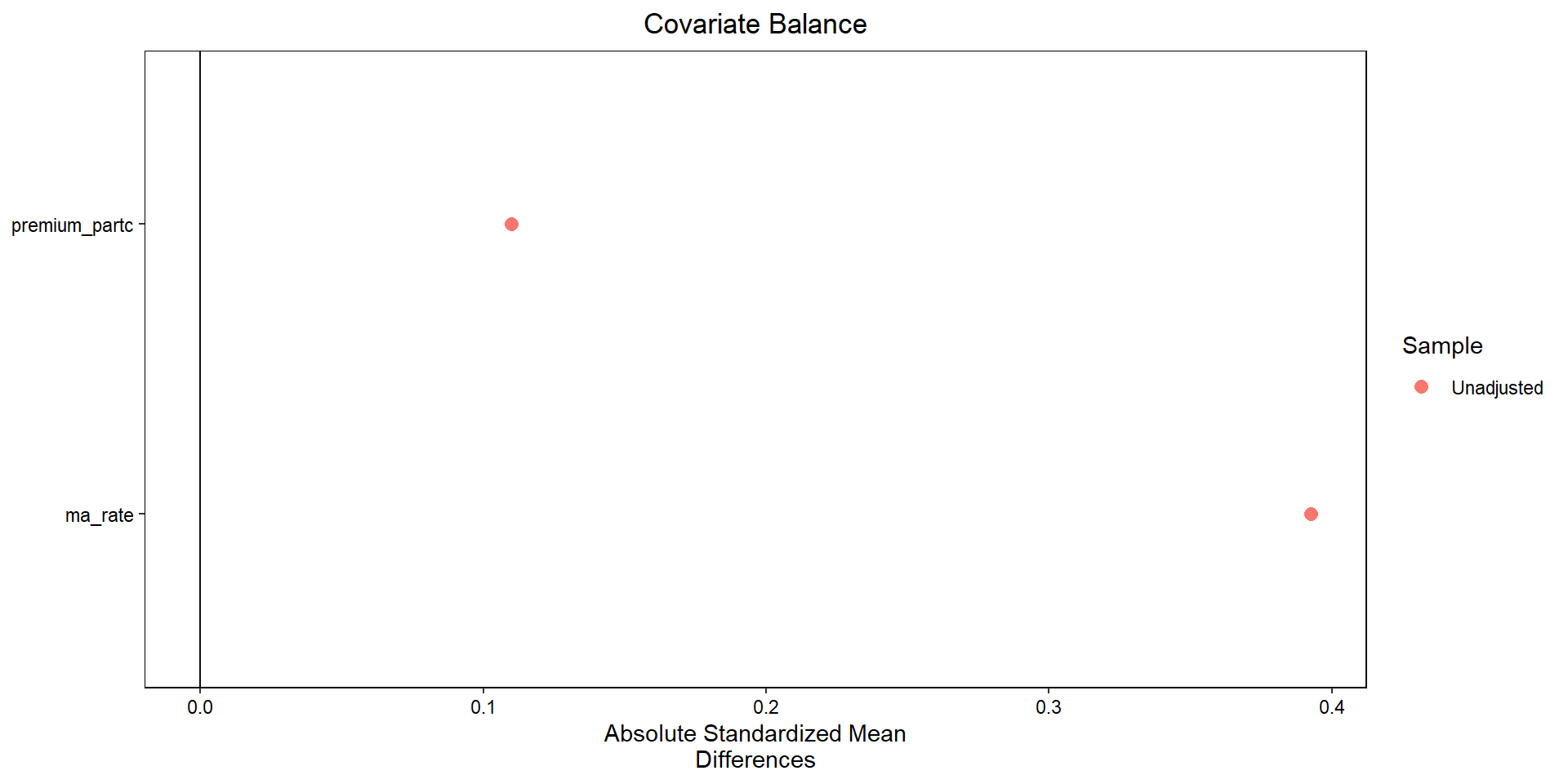
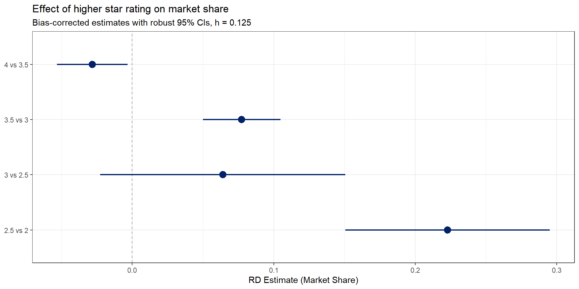
Effects across all thresholds
Same approach, applied to every half-star cutoff. The code below loops over each threshold and collects the rdrobust estimates into a single data frame.
cutoffs <- tibble(
  lower = c(2, 2.5, 3, 3.5),
  upper = c(2.5, 3, 3.5, 4),
  cutoff = c(2.25, 2.75, 3.25, 3.75)
)

rd_results <- cutoffs %>%
  pmap_dfr(function(lower, upper, cutoff) {
    dat <- ma_2009 %>%
      filter(Star_Rating == lower | Star_Rating == upper) %>%
      mutate(score = raw_rating - cutoff)

    est <- rdrobust(y=dat$mkt_share, x=dat$score, c=0,
                    h=0.125, p=1, kernel="uniform", vce="hc0",
                    masspoints="off")

    tibble(
      threshold = paste0(upper, " vs ", lower),
      estimate = est$coef[2],
      ci_lower = est$ci[3,1],
      ci_upper = est$ci[3,2],
      n = est$N[1] + est$N[2]
    )
  })
from rdrobust import rdrobust
import pandas as pd
cutoffs = [
(2, 2.5, 2.25),
(2.5, 3, 2.75),
(3, 3.5, 3.25),
(3.5, 4, 3.75),
]
results = []
for lower, upper, cutoff in cutoffs:
dat = ma_2009[ma_2009["Star_Rating"].isin([lower, upper])].copy()
dat["score"] = dat["raw_rating"] - cutoff
est = rdrobust(
y=dat["mkt_share"].values,
x=dat["score"].values,
c=0, h=0.125, p=1,
kernel="uniform", vce="hc0",
masspoints="off"
)
results.append({
"threshold": f"{upper} vs {lower}",
"estimate": est.coef.iloc[1, 0], # bias-corrected
"ci_lower": est.ci.iloc[2, 0], # robust CI
"ci_upper": est.ci.iloc[2, 1],
})
rd_results = pd.DataFrame(results)