Instrumental Variables: Part II

Ian McCarthy | Emory University

Outline for Today

1. HRRP Penalties and Pricing
2. IV in Practice

Organize Data

First we need to organize the data into something we can analyze with IV in this setting

• Reduce to cross-sectional data (we’ll deal with panel data in the next module)
• Focus on price changes, not levels
• Maintain Medicare discharges as our key instrument

• R
• Python
• Output

hcris.data <- read_csv("../data/output/hcris-snippets/hcris-data.csv")

hcris.price <- hcris.data %>%
  filter(year %in% c(2011, 2014)) %>%
  select(provider_number, price, year) %>%
  pivot_wider(names_from=year, values_from=price, names_prefix="price_")

hcris.hrrp <- hcris.data %>%
  filter(year==2012) %>%
  mutate(hrrp_penalty=if_else(hrrp_payment>0 & !is.na(hrrp_payment), hrrp_payment/1000, 0)) %>%
  select(provider_number, hrrp_penalty) %>%
  mutate(any_penalty=(hrrp_penalty>0))

hcris.mcare <- hcris.data %>%
  filter(year<2012) %>%
  group_by(provider_number) %>%
  summarize(avg_mcare=mean(mcare_discharges, na.rm=TRUE)/100) %>%
  ungroup()

hcris.final <- hcris.price %>%
  left_join(hcris.hrrp, by="provider_number") %>%
  left_join(hcris.mcare, by="provider_number") %>%
  filter(!is.na(price_2011), !is.na(price_2014)) %>%
  mutate(price_change=price_2014-price_2011)

import pandas as pd
import numpy as np

# read
hcris_data = pd.read_csv("../data/output/hcris-snippets/hcris-data.csv")

# --- prices (wide) ---
hcris_price = (
    hcris_data.loc[hcris_data["year"].isin([2011, 2014]), ["provider_number", "price", "year"]]
    .pivot(index="provider_number", columns="year", values="price")
    .rename(columns=lambda y: f"price_{int(y)}")
    .reset_index()
)

# --- HRRP (2012) ---
hcris_hrrp = (
    hcris_data.loc[hcris_data["year"].eq(2012), ["provider_number", "hrrp_payment"]]
    .assign(
        hrrp_penalty=lambda df: np.where(
            (df["hrrp_payment"] > 0) & df["hrrp_payment"].notna(),
            df["hrrp_payment"] / 1000,   # $1000s
            0.0
        )
    )
    .loc[:, ["provider_number", "hrrp_penalty"]]
    .assign(any_penalty=lambda df: df["hrrp_penalty"] > 0)
)

# --- Medicare discharges instrument: avg pre-2012 ---
hcris_mcare = (
    hcris_data.loc[hcris_data["year"] < 2012, ["provider_number", "mcare_discharges"]]
    .groupby("provider_number", as_index=False)
    .agg(avg_mcare=("mcare_discharges", lambda x: np.nanmean(x) / 100))
)

# --- final merge + long difference outcome ---
hcris_final = (
    hcris_price
    .merge(hcris_hrrp, on="provider_number", how="left")
    .merge(hcris_mcare, on="provider_number", how="left")
)

hcris_final = (
    hcris_final.loc[hcris_final["price_2011"].notna() & hcris_final["price_2014"].notna()]
    .assign(price_change=lambda df: df["price_2014"] - df["price_2011"])
)

# A tibble: 6 × 7
  provider_number price_2011 price_2014 hrrp_penalty any_penalty avg_mcare
  <chr>                <dbl>      <dbl>        <dbl> <lgl>           <dbl>
1 010001               4476.      5361.            0 FALSE            79.8
2 010005               1327.      1557.            0 FALSE            22.3
3 010006               4612.      4604.            0 FALSE            51.9
4 010007                840.       423.            0 FALSE            10.8
5 010011               8310.      5159.            0 FALSE            41.8
6 010012               6774.      6414.            0 FALSE            17.4
# ℹ 1 more variable: price_change <dbl>

Understanding this Dataset

• Difference prices to remove time-invariant hospital characteristics
• Can then estimate a cross-sectional IV model where cumulative HRRP penalties are instrumented using pre-period Medicare volume
• Sometimes referred to as IV with long-differenced outcomes

Why Price Differences (instead of levels)?

• Assume a simple two-period model for hospital \(i\) in years \(t \in \{2011, 2014\}\): \[p_{it} = \beta\,\text{pen}_{i,t-2} + \alpha_i + u_{it},\] where \(\alpha_i\) is a time-invariant hospital fixed effect (e.g., hospital 1 is just different than hospital 2 in some time-invariant way).

• Take the long difference (2014 minus 2011): \(\Delta p_i \equiv p_{i,2014}-p_{i,2011}.\)

• Substitute the model into both terms and difference: \[\Delta p_i= \beta(\text{pen}_{i,2012}-\text{pen}_{i,2009}) + (\alpha_i-\alpha_i) + (u_{i,2014}-u_{i,2011}).\]

• Because \(\alpha_i\) does not change over time, it cancels: \[(\alpha_i-\alpha_i)=0 \quad \Rightarrow \quad \Delta p_i = \beta\,\Delta \text{pen}_i + \Delta u_i.\]

• Differencing removes any time-invariant hospital-level confounder captured by \(\alpha_i\).

• Time-varying hospital shocks remain in \(\Delta u_i\).

Naive OLS Estimate

Before moving to IV, let’s look first at a simple OLS estimate, ignoring any potential endogeneity problems

• R
• Python
• Output

lm(price_change~hrrp_penalty, data=hcris.final)

import statsmodels.formula.api as smf

ols = smf.ols("price_change ~ hrrp_penalty", data=hcris_final).fit()
print(ols.summary())

Call:
lm(formula = price_change ~ hrrp_penalty, data = hcris.final)

Residuals:
    Min      1Q  Median      3Q     Max 
-884980   -1338    -142    1170  880921 

Coefficients:
             Estimate Std. Error t value Pr(>|t|)
(Intercept)   276.798    525.707   0.527    0.599
hrrp_penalty    4.562     15.707   0.290    0.771

Residual standard error: 25450 on 2512 degrees of freedom
  (5 observations deleted due to missingness)
Multiple R-squared:  3.359e-05, Adjusted R-squared:  -0.0003645 
F-statistic: 0.08438 on 1 and 2512 DF,  p-value: 0.7715

Is this causal?

Lots of reasons some hospitals might be penalized versus others. Any ideas?

Instrumental Variables in Practice

Medicare Discharges (at baseline) as an IV

• R
• Python
• Output

mcare.hrrp.plot <- ggplot(hcris.final, aes(x = avg_mcare, y = hrrp_penalty)) +
  geom_point(alpha = 0.6) +
  labs(
    x = "Medicare Discharges (before 2012) in 100s",
    y = "HRRP Penalty (2012) in thousands $",
    title = "HRRP Penalties vs Pre-Period Medicare Volume"
  ) +
  theme_bw()

import matplotlib.pyplot as plt

plt.figure()
plt.scatter(
    hcris_final["avg_mcare"],
    hcris_final["hrrp_penalty"],
    alpha=0.6
)

plt.xlabel("Medicare Discharges (before 2012) in 100s")
plt.ylabel("HRRP Penalty (2012) in thousands $")
plt.title("HRRP Penalties vs Pre-Period Medicare Volume")

plt.show()

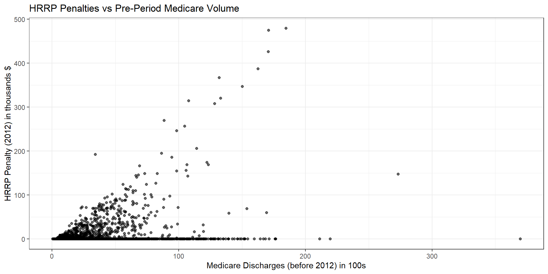
Assessment of Instrument

Before looking at IV results, Let’s examine the first-stage and the reduced form:

• R
• Python
• Output

first.stage <- feols(hrrp_penalty ~ avg_mcare, data=hcris.final)
red.form <- feols(price_change ~ avg_mcare, data=hcris.final)

modelsummary(list("First Stage"=first.stage, "Reduced Form"=red.form),
          keep=c("avg_mcare"),
          coef_map=c("avg_mcare"="Pre-HRRP Medicare Discharges"),
          gof_map=c("nobs", "r.squared"))

import statsmodels.formula.api as smf

# first stage
first_stage = smf.ols("hrrp_penalty ~ avg_mcare", data=hcris_final).fit()

# reduced form
red_form = smf.ols("price_change ~ avg_mcare", data=hcris_final).fit()

print(first_stage.summary())
print(red_form.summary())

import pandas as pd

table = pd.DataFrame({
    "First Stage": [
        first_stage.params["avg_mcare"],
        first_stage.bse["avg_mcare"],
        first_stage.nobs,
        first_stage.rsquared
    ],
    "Reduced Form": [
        red_form.params["avg_mcare"],
        red_form.bse["avg_mcare"],
        red_form.nobs,
        red_form.rsquared
    ]
},
index=[
    "Pre-HRRP Medicare Discharges",
    "Std. Error",
    "N",
    "R-squared"
])

print(table)

	First Stage	Reduced Form
Pre-HRRP Medicare Discharges	0.322	38.450
	(0.019)	(16.091)
Num.Obs.	2514	2519
R2	0.098	0.002

• Sign of reduced form in the expected direction
• First-stage coefficient is positive, with F-stat of nearly 290

IV Results

• Now time to implement “official” IV estimator
• Note…\(R^2\) no longer relevant measure of model fit for IV as the standard variance decomposition no longer holds
• Note also…I’m not worried here about statistical inference (standard errors are likely wrong and would be larger under heteroskedasticity and smaller when considering a “richer” specification)

• R
• Python
• Output

ols <- feols(price_change ~ hrrp_penalty, data=hcris.final)
iv <- feols(price_change ~ 1 | hrrp_penalty~avg_mcare, data=hcris.final)

modelsummary(list("OLS"=ols, "IV"=iv),
          keep=c("hrrp_penalty"),
          coef_map=c("hrrp_penalty"="HRRP Penalty ($1000s)", "fit_hrrp_penalty"="HRRP Penalty ($1000s)"),
          gof_map=c("nobs"))

import pandas as pd
import statsmodels.formula.api as smf

# --- OLS ---
ols = smf.ols("price_change ~ hrrp_penalty", data=hcris_final).fit()

# --- IV / 2SLS (linearmodels is the closest analogue to fixest IV) ---
from linearmodels.iv import IV2SLS

iv = IV2SLS.from_formula(
    "price_change ~ 1 + [hrrp_penalty ~ avg_mcare]",
    data=hcris_final
).fit(cov_type="robust")

print(ols.summary())
print(iv.summary)

# --- modelsummary-like table (coef, SE, N only) ---
out = pd.DataFrame(
    {
        "OLS": {
            "HRRP Penalty ($1000s)": ols.params["hrrp_penalty"],
            "Std. Error": ols.bse["hrrp_penalty"],
            "N": int(ols.nobs),
        },
        "IV": {
            "HRRP Penalty ($1000s)": iv.params["hrrp_penalty"],
            "Std. Error": iv.std_errors["hrrp_penalty"],
            "N": int(iv.nobs),
        },
    }
)

print(out)

	OLS	IV
HRRP Penalty ($1000s)	4.562	119.026
	(15.707)	(50.580)
Num.Obs.	2514	2514

Some other IV issues

1. IV estimators are biased. Performance in finite samples is questionable.
2. IV estimators provide an estimate of a Local Average Treatment Effect (LATE), which is only the same as the ATT under strong conditions or assumptions.
3. What about lots of instruments? The finite sample problem is more important and we may try other things (JIVE).

The National Bureau of Economic Researh (NBER) has a great resource here for understanding instruments in practice.

Quick IV Review

1. When do we consider IV as a potential identification strategy?
2. What are the main IV assumptions (and what do they mean)?
3. How do we test those assumptions?