hcris.data <- read_csv("../data/output/hcris-snippets/hcris-data.csv") %>%
  mutate(
    expand_year = lubridate::year(date_adopted),
    expand_ever = expanded,
    status = if_else(!is.na(expand_year) & year >= expand_year, "Expanded", "Not Expanded"),
    uncomp_care_m = uncomp_care / 1e6
  ) %>%
  filter(!is.na(expand_ever))

uc.plot.dat <- hcris.data %>%
  group_by(expand_ever, year) %>%
  summarize(mean = mean(uncomp_care_m, na.rm = TRUE), .groups = "drop")

uc.plot <- ggplot(data = uc.plot.dat, aes(x = year, y = mean, group = expand_ever, linetype = expand_ever)) +
  geom_line() + geom_point() + theme_bw() +
  geom_vline(xintercept = 2013.5, color = "red") +
  geom_text(data = uc.plot.dat %>% filter(year == 2015),
            aes(label = c("Non-expansion", "Expansion"),
                x = year + 1,
                y = mean)) +
  guides(linetype = "none") +
  labs(
    x = "Year",
    y = "Uncompensated Care ($mm)",
    title = "Hospital Uncompensated Care Over Time"
)Difference-in-differences Part II
Step 1: Look at the data
import pandas as pd
import numpy as np
import matplotlib.pyplot as plt

hcris_data = pd.read_csv("../data/output/hcris-snippets/hcris-data.csv")

hcris_data["expand_year"] = pd.to_datetime(hcris_data["date_adopted"]).dt.year
hcris_data["expand_ever"] = hcris_data["expanded"]

hcris_data["status"] = np.where(
    (~hcris_data["expand_year"].isna()) & (hcris_data["year"] >= hcris_data["expand_year"]),
    "Expanded",
    "Not Expanded"
)

hcris_data["uncomp_care_m"] = hcris_data["uncomp_care"] / 1_000_000

hcris_data = hcris_data.loc[~hcris_data["expand_ever"].isna()].copy()

uc_plot_dat = (
    hcris_data
    .groupby(["expand_ever", "year"], as_index=False)
    .agg(mean=("uncomp_care_m", "mean"))
)

# Example plot in Python (kept minimal since output is shown from R)
for key, grp in uc_plot_dat.groupby("expand_ever"):
    plt.plot(grp["year"], grp["mean"], marker="o", label=str(key))

plt.axvline(2013.5, color="red")
plt.xlabel("Year")
plt.ylabel("Uncompensated Care ($mm)")
plt.title("Hospital Uncompensated Care Over Time")
plt.legend()
plt.show()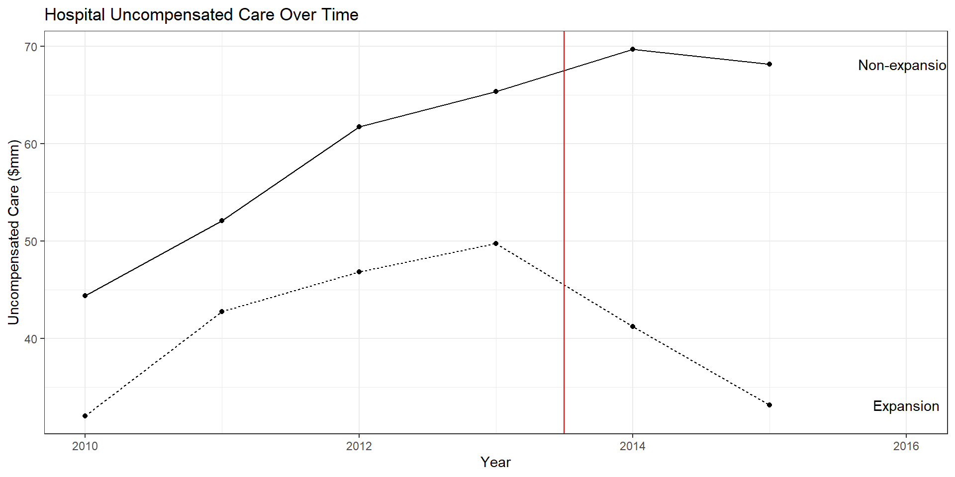
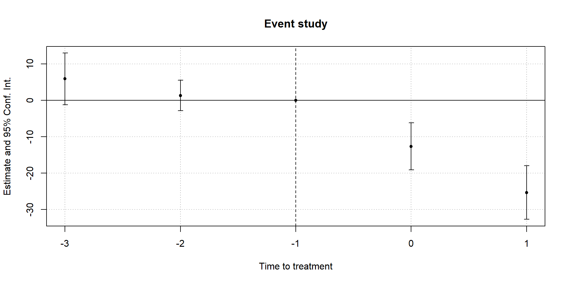
Common treatment timing
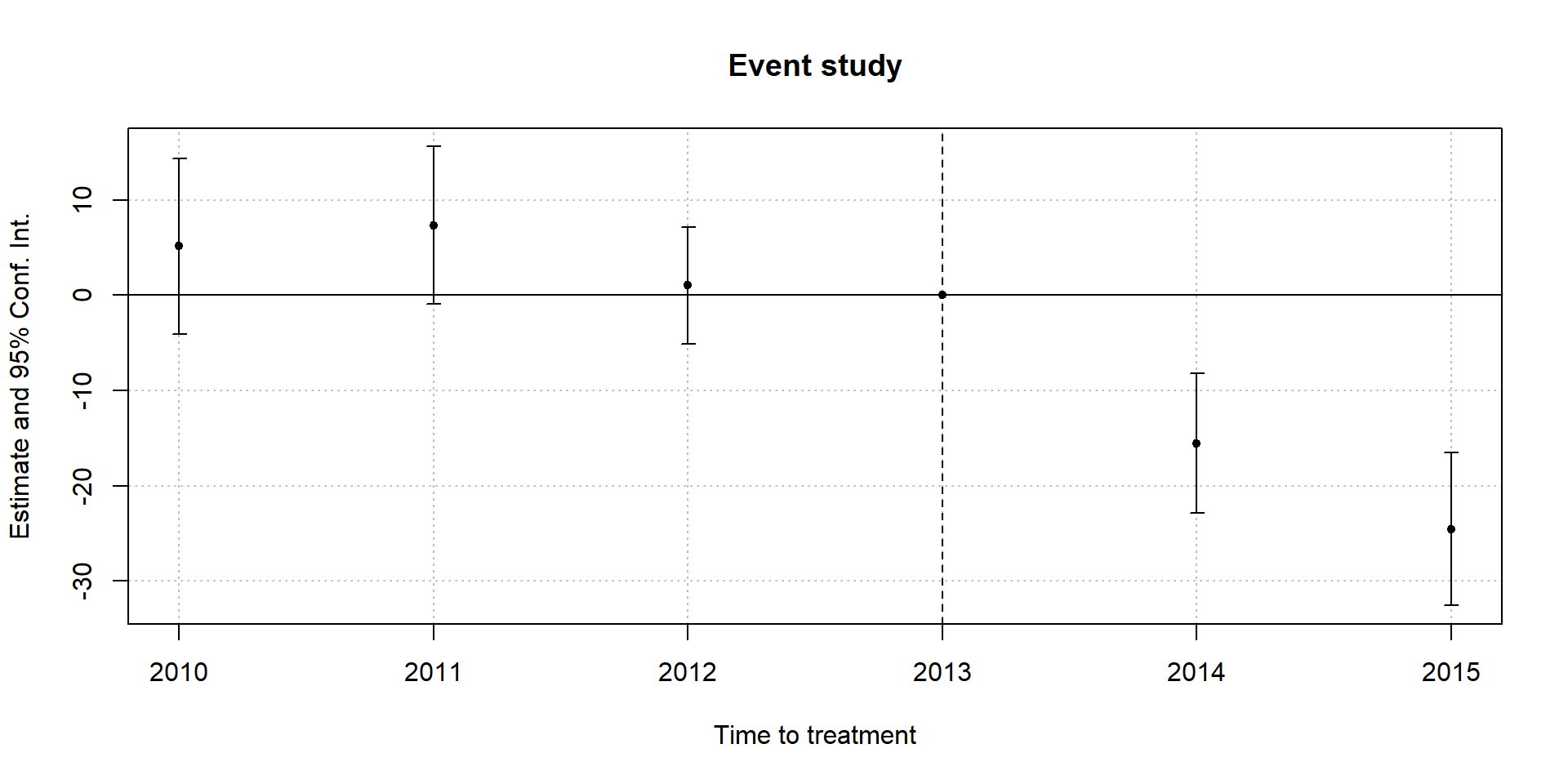
Differential treatment timing
reg.dat.full <- hcris.data %>%
  filter(!is.na(expand_ever)) %>%
  mutate(
    time_to_treat = if_else(expand_ever == FALSE, 0, year - expand_year),
    time_to_treat = if_else(time_to_treat < -3, -3, time_to_treat)
  )

mod.twfe.full <- feols(uncomp_care_m ~ i(time_to_treat, expand_ever, ref = -1) | provider_number + year,
                       cluster = ~ state,
                       data = reg.dat.full)
reg_dat_full = hcris_data.loc[~hcris_data["expand_ever"].isna()].copy()
reg_dat_full["time_to_treat"] = np.where(
reg_dat_full["expand_ever"].astype(bool),
reg_dat_full["year"] - reg_dat_full["expand_year"],
0
)
reg_dat_full["time_to_treat"] = reg_dat_full["time_to_treat"].clip(lower=-3)
mod_twfe_full = smf.ols(
"uncomp_care_m ~ C(time_to_treat)*expand_ever + C(provider_number) + C(year)",
data=reg_dat_full
).fit()
print(mod_twfe_full.summary())