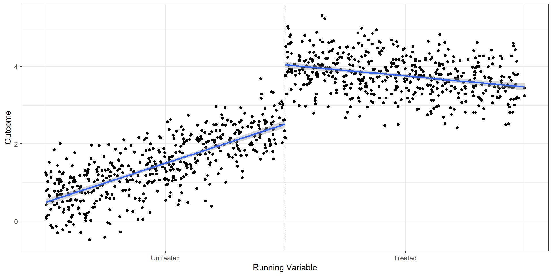
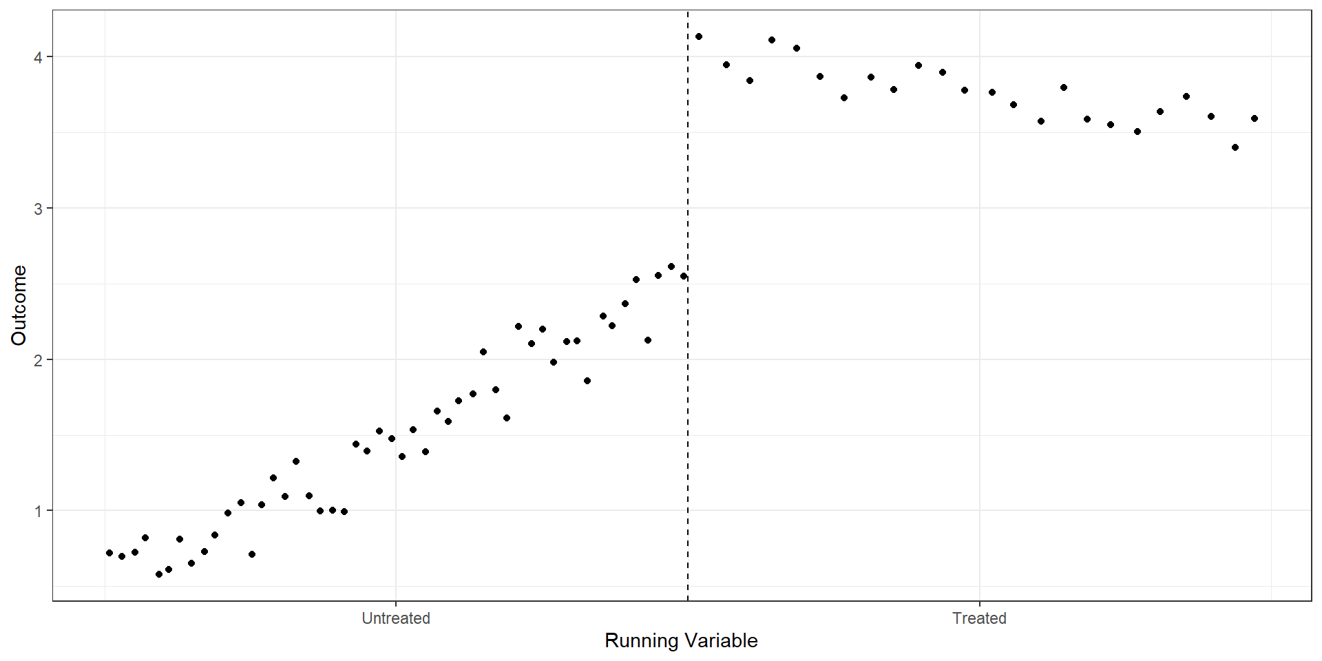
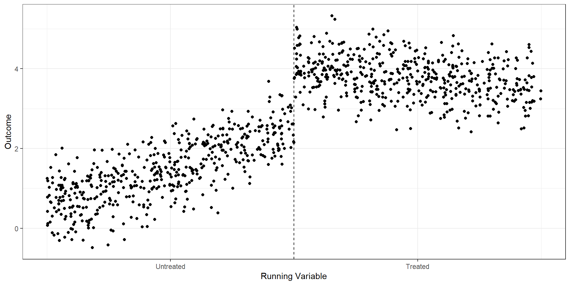
Regression Discontinuity: Part I

Ian McCarthy | Emory University

Motivation

Motivation

Highly relevant in “rule-based” world…

  • School eligibility based on age cutoffs
  • Program participation based on discrete income thresholds
  • Performance scores rounded to nearest integer

Required elements

  1. Score
  2. Cutoff
  3. Treatment

Types of RD

  1. Sharp regression discontinuity: those above the threshold guaranteed to participate<
  2. Fuzzy regression discontinuity: those above the threshold are eligible but may not participate

Sharp RD

\[W_{i} = 1(x_{i}>c) = \begin{cases} 1 & \text{if} & x_{i}>c \\ 0 & \text{if} & x_{i}<c \end{cases}\]

  • \(x\) is “forcing variable”
  • \(c\) is the threshold value or cutoff point

Sharp RD Scatterplot

R Code
n=1000
rd.dat <- tibble(
  X = runif(n,0,2),
  W = (X>1),
  Y = 0.5 + 2*X + 4*W + -2.5*W*X + rnorm(n,0,.5)
)
plot1 <- rd.dat %>% ggplot(aes(x=X,y=Y)) + 
  geom_point() + theme_bw() +
  geom_vline(aes(xintercept=1),linetype='dashed') +
  scale_x_continuous(
    breaks = c(.5, 1.5),
    label = c("Untreated", "Treated")
  ) +
  xlab("Running Variable") + ylab("Outcome")
plot1

Sharp RD Linear Predictions

R Code
plot2 <- plot1 +
  geom_smooth(method = 'lm', data = (rd.dat %>% filter(W == TRUE)) ) +
  geom_smooth(method = 'lm', data = (rd.dat %>% filter(W == FALSE)) )
plot2

Sharp RD Linear Predictions

R Code
plot3 <- plot2 +
  stat_smooth(method = 'lm', data = (rd.dat %>% filter(W == TRUE)), fullrange = TRUE, linetype = 'dashed') +
  stat_smooth(method = 'lm', data = (rd.dat %>% filter(W == FALSE)), fullrange = TRUE, linetype = 'dashed')
plot3

Different averages

  • Mean difference around threshold of 0.2, 3.94 - 2.24 = 1.7
  • Mean overall difference, 3.75 - 1.45 = 2.29

More generally

  • Running variable may affect outcome directly
  • Focusing on area around cutoff does two things:
  1. Controls for running variable
  2. “Controls” for unobserved things correlated with running variable and outcome

Animations!

Estimation

Goal is to estimate \(E[Y_{1}|X=c] - E[Y_{0}|X=c]\)

  1. Trim to reasonable window around threshold (“bandwidth”), \(X \in [c-h, c+h]\)
  2. Transform running variable, \(\tilde{X}=X-c\)
  3. Estimate regressions…
  • Linear, same slope: \(y = \alpha + \delta D + \beta \tilde{X} + \varepsilon\)
  • Linear, different slope: \(y = \alpha + \delta D + \beta \tilde{X} + \gamma W\tilde{X} + \varepsilon\)
  • Nonlinear: add polynomials in \(\tilde{X}\) and interactions \(W \tilde{X}\)

Regression Discontinuity in Practice

RDs “in the wild”

Most RD estimates follow a similar set of steps:

  1. Show clear graphical evidence of a change around the discontinuity (bin scatter)
  2. Balance above/below threshold (use baseline covariates as outcomes)
  3. Manipulation tests
  4. RD estimates
  5. Sensitivity and robustness:
    • Bandwidths
    • Order of polynomial
    • Inclusion of covariates

1. Graphical evidence

Before presenting RD estimates, any good RD approach first highlights the discontinuity with a simple graph. We can do so by plotting the average outcomes within bins of the forcing variable (i.e., binned averages), \[\bar{Y}_{k} = \frac{1}{N_{k}}\sum_{i=1}^{N} Y_{i} \times 1(b_{k} < X_{i} \leq b_{k+1}).\]

The binned averages helps to remove noise in the graph and can provide a cleaner look at the data. Just make sure that no bin includes observations above and below the cutoff!

Binned average calculation

R Code
library(rdrobust)
rd.result <- rdplot(rd.dat$Y, rd.dat$X, 
                    c=1, 
                    title="RD Plot with Binned Average", 
                    x.label="Running Variable", 
                    y.label="Outcome")
R Code
bin.avg <- as_tibble(rd.result$vars_bins)
plot.bin <- bin.avg %>% ggplot(aes(x=rdplot_mean_x,y=rdplot_mean_y)) + 
  geom_point() + theme_bw() +
  geom_vline(aes(xintercept=1),linetype='dashed') +
  scale_x_continuous(
    breaks = c(.5, 1.5),
    label = c("Untreated", "Treated")
  ) +
  xlab("Running Variable") + ylab("Outcome")

With and without binning

Selecting “bin” width

  1. Dummy variables: Create dummies for each bin, regress the outcome on the set of all dummies and form r-square \(R^{2}_{r}\), repeat with double the number of bins and find r-square value \(R^{2}_{u}\), form F-stat, \(\frac{R^{2}_{u}-R^{2}_{r}}{1-R^{2}_{u}}\times \frac{n-K-1}{K}\).

  2. Interaction terms: Include interactions between dummies and the running variable, joint F-test for the interaction terms

If F-test suggests significance, then we have too few bins and need to narrow the bin width.

2. Balance

  • If RD is an appropriate design, passing the cutoff should only affect treatment and outcome of interest
  • How do we test for this?
    • Covariate balance
    • Placebo tests of other outcomes (e.g., t-1 outcomes against treatment at time t)

3. Manipulation tests

  • Individuals should not be able to precisely manipulate running variable to enter into treatment
  • Sometimes discussed as “bunching”
  • Test for differences in density to left and right of cutoffs (rddensity in Stata and R)
  • Permutation tests proposed in Ganong and Jager (2017)

Bunching?

  • Gerard, Rokkanen, and Rothe (2020) suggest partial identification allowing for bunching
  • Can also be used as a robustness check
  • rdbounds in Stata and R
  • Assumption: bunching only moves people in one direction

4. RD Estimation

Start with the “default” options

  • Local linear regression
  • Optimal bandwidth
  • Uniform kernel

Selecting bandwidth in local linear regression

The bandwidth is a “tuning parameter”

  • High \(h\) means high bias but lower variance (use more of the data, closer to OLS)
  • Low \(h\) means low bias but higher variance (use less data, more focused around discontinuity)

Represent bias-variance tradeoff with the mean-square error, \[MSE(h) = E[(\hat{\tau}_{h} - \tau_{RD})^2]=\left(E[\hat{\tau}_{h} - \tau_{RD}] \right)^2 + V(\hat{\tau}_{h}).\]

Selecting bandwidth

In the RD case, we have two different mean-square error terms:

  1. “From above”, \(MSE_{+}(h) = E[(\hat{\mu}_{+}(c,h) - E[Y_{1i}|X_{i}=c])^2]\)
  2. “From below”, \(MSE_{-}(h) = E[(\hat{\mu}_{-}(c,h) - E[Y_{0i}|X_{i}=c])^2]\)

Goal is to find \(h\) that minimizes these values, but we don’t know the true \(E[Y_{1}|X=c]\) and \(E[Y_{0}|X=c]\). So we have two approaches:

  1. Use cross-validation to choose \(h\)
  2. Explicitly solve for optimal bandwidth

Cross-validation

Essentially a series of “leave-one-out” estimates:

  1. Pick an \(h\)
  2. Run regression, leaving out observation \(i\). If \(i\) is to the left of the threshold, we estimate regression for observations within \(X_{i}-h\), and conversely \(X_{i}+h\) if \(i\) is to the right of the threshold.
  3. Predicted \(\hat{Y}_{i}\) at \(X_{i}\) (out of sample prediction for the left out observation)
  4. Do this for all \(i\), and form \(CV(h)=\frac{1}{N}\sum (Y_{i} - \hat{Y}_{i})^2\)

Select \(h\) with lowest \(CV(h)\) value.

Back to simulated data

R Code
rd.dat %>% ggplot(aes(x=X,y=Y)) + 
  geom_point() + theme_bw() +
  geom_vline(aes(xintercept=1),linetype='dashed') +
  scale_x_continuous(
    breaks = c(.5, 1.5),
    label = c("Untreated", "Treated")
  ) +
  xlab("Running Variable") + ylab("Outcome")

Back to simulated data

R Code
ols <- lm(Y~X+W, data=rd.dat)

rd.dat3 <- rd.dat %>%
  mutate(x_dev = X-1) %>%
  filter( (X>0.8 & X <1.2) )
rd <- lm(Y~x_dev + W, data=rd.dat3)
  • True effect: 1.5
  • Standard linear regression with same slopes: 1.51
  • RD (linear with same slopes): 1.18

RD with built-in commands

R Code
rd.y <- rd.dat$Y
rd.x <- rd.dat$X
rd.est <- rdrobust(y=rd.y, x=rd.x, c=1)
summary(rd.est)
Sharp RD estimates using local polynomial regression.

Number of Obs.                 1000
BW type                       mserd
Kernel                   Triangular
VCE method                       NN

Number of Obs.                  504          496
Eff. Number of Obs.             159          144
Order est. (p)                    1            1
Order bias  (q)                   2            2
BW est. (h)                   0.326        0.326
BW bias (b)                   0.568        0.568
rho (h/b)                     0.574        0.574
Unique Obs.                     504          496

=============================================================================
        Method     Coef. Std. Err.         z     P>|z|      [ 95% C.I. ]       
=============================================================================
  Conventional     1.327     0.122    10.899     0.000     [1.089 , 1.566]     
        Robust         -         -     9.145     0.000     [1.009 , 1.559]     
=============================================================================

Cattaneo et al. (2020) argue: - Report conventional point estimate - Report robust confidence interval

5. Robustness and sensitivity

  • Different bandwidths
  • Different kernels or polynomials
  • Role of covariates in RD estimates

Pitfalls of polynomials

  • Assign too much weight to points away from the cutoff
  • Results highly sensitive to degree of polynomial
  • Narrow confidence intervals (over-rejection of the null)

For more discussion, see this World Bank Blog post

Fuzzy RD

The Idea

“Fuzzy” just means that assignment isn’t guaranteed based on the running variable. For example, maybe students are much more likely to get a scholarship past some threshold SAT score, but it remains possible for students below the threshold to still get the scholarship.

  • Discontinuity reflects a jump in the probability of treatment
  • Other RD assumptions still required (namely, can’t manipulate running variable around the threshold)

Fuzzy RD is IV

In practice, fuzzy RD is employed as an instrumental variables estimator

  • Difference in outcomes among those above and below the discontinuity divided by the difference in treatment probabilities for those above and below the discontinuity,
    \(E[Y_{i} | D_{i}=1] - E[Y_{i} | D_{i}=0] = \frac{E[Y_{i} | x_{i}\geq c] - E[Y_{i} | x_{i}< c]}{E[D_{i} | x_{i}\geq c] - E[D_{i} | x_{i}<c]}\)
  • Indicator for \(x_{i}\geq c\) is an instrument for treatment status, \(D_{i}\).
  • Implemented with rdrobust and fuzzy=t option