Understanding Difference-in-differences
Outline
- Panel Data and Fixed Effects
- Difference-in-Differences
Panel Data and Fixed Effects
Basics of panel data
- Repeated observations of the same units over time (balanced vs unbalanced)
- Identification due to variation within unit
Notation
- Unit \(i=1,...,N\) over several periods \(t=1,...,T\), which we denote \(y_{it}\)
- Treatment status \(D_{it}\)
- Regression model,
\(y_{it} = \delta D_{it} + \gamma_{i} + \gamma_{t} + \epsilon_{it}\) for \(t=1,...,T\) and \(i=1,...,N\)
Benefits of Panel Data
- May overcome certain forms of omitted variable bias
- Allows for unobserved but time-invariant factor, \(\gamma_{i}\), that affects both treatment and outcomes
Still assumes
- No time-varying confounders
- Past outcomes do not directly affect current outcomes
- Past outcomes do not affect treatment (reverse causality)
Some textbook settings
- Unobserved “ability” when studying schooling and wages
- Unobserved “quality” when studying physicians or hospitals
Fixed effects and regression
\(y_{it} = \delta D_{it} + \gamma_{i} + \gamma_{t} + \epsilon_{it}\) for \(t=1,...,T\) and \(i=1,...,N\)
- Allows correlation between \(\gamma_{i}\) and \(D_{it}\)
- Physically estimate \(\gamma_{i}\) in some cases via set of dummy variables
- More generally, “remove” \(\gamma_{i}\) via:
- “within” estimator
- first-difference estimator
Within Estimator
\(y_{it} = \delta D_{it} + \gamma_{i} + \gamma_{t} + \epsilon_{it}\) for \(t=1,...,T\) and \(i=1,...,N\)
Most common approach (default in most statistical software)
Equivalent to demeaned model: \[y_{it} - \bar{y}_{i} = \delta (D_{it} - \bar{D}_{i}) + (\gamma_{i} - \bar{\gamma}_{i}) + (\gamma_{t} - \bar{\gamma}_{t}) + (\epsilon_{it} - \bar{\epsilon}_{i})\]
\(\gamma_{i} - \bar{\gamma}_{i} = 0\) since \(\gamma_{i}\) is time-invariant
Requires strict exogeneity assumption (error is uncorrelated with \(D_{it}\) for all time periods)
First-difference
\(y_{it} = \delta D_{it} + \gamma_{i} + \gamma_{t} + \epsilon_{it}\) for \(t=1,...,T\) and \(i=1,...,N\)
Instead of subtracting the mean, subtract the prior period values \[y_{it} - y_{i,t-1} = \delta(D_{it} - D_{i,t-1}) + (\gamma_{i} - \gamma_{i}) + (\gamma_{t} - \gamma_{t-1}) + (\epsilon_{it} - \epsilon_{i,t-1})\]
Requires exogeneity of \(\epsilon_{it}\) and \(D_{it}\) only for time \(t\) and \(t-1\) (weaker assumption than within estimator)
Sometimes useful to estimate both FE and FD just as a check
Keep in mind…
- Discussion only applies to linear case or very specific nonlinear models
- Fixed effects at lower “levels” accommodate fixed effects at higher levels (e.g., FEs for hospital combine to form FEs for zip code, etc.)
- Fixed effects can’t solve reverse causality
- Fixed effects don’t address unobserved, time-varying confounders
- Can’t estimate effects on time-invariant variables
- May “absorb” a lot of the variation for variables that don’t change much over time
Within Estimator (Default) in practice
Within Estimator (Default) in practice
R Code
library(fixest)
library(modelsummary)
library(causaldata)
reg.dat <- causaldata::gapminder %>%
  mutate(lgdp_pc=log(gdpPercap))
m1 <- feols(lifeExp ~ lgdp_pc | country, data=reg.dat)
modelsummary(list("Default FE"=m1),
             shape=term + statistic ~ model,
             gof_map=NA,
coef_rename=c("lgdp_pc"="Log GDP per Capita"))| Default FE | |
|---|---|
| Log GDP per Capita | 9.769 |
| (0.702) |
Within Estimator (Manually Demean) in practice
Within Estimator (Manually Demean) in practice
R Code
library(lmtest)
reg.dat <- causaldata::gapminder %>%
  group_by(country) %>%
  mutate(lgdp_pc=log(gdpPercap),
         lgdp_pc=lgdp_pc - mean(lgdp_pc, na.rm=TRUE),
         lifeExp=lifeExp - mean(lifeExp, na.rm=TRUE))

m2 <- lm(lifeExp~ 0 + lgdp_pc , data=reg.dat)
modelsummary(list("Default FE"=m1, "Manual FE"=m2),
             shape=term + statistic ~ model,
             gof_map=NA,
             coef_rename=c("lgdp_pc"="Log GDP per Capita"),
vcov = ~country)| Default FE | Manual FE | |
|---|---|---|
| Log GDP per Capita | 9.769 | 9.769 |
| (0.702) | (0.701) |
Note: feols defaults to clustering at level of FE, lm requires our input
First differencing (default) in practice
First differencing (manual) in practice
R Code
library(plm)
reg.dat <- causaldata::gapminder %>%
  mutate(lgdp_pc=log(gdpPercap))

m3 <- plm(lifeExp ~ 0 + lgdp_pc, model="fd", index=c("country","year"), data=reg.dat)

modelsummary(list("Default FE"=m1, "Manual FE"=m2, "Default FD"=m3),
             shape=term + statistic ~ model,
             gof_map=NA,
coef_rename=c("lgdp_pc"="Log GDP per Capita"))| Default FE | Manual FE | Default FD | |
|---|---|---|---|
| Log GDP per Capita | 9.769 | 9.769 | 5.290 |
| (0.702) | (0.284) | (0.291) |
First differencing (manual) in practice
First differencing (manual) in practice
R Code
reg.dat <- causaldata::gapminder %>%
  mutate(lgdp_pc=log(gdpPercap)) %>%
  group_by(country) %>%
  arrange(country, year) %>%
  mutate(fd_lifeexp=lifeExp - dplyr::lag(lifeExp),
         lgdp_pc=lgdp_pc - dplyr::lag(lgdp_pc)) %>%
  na.omit()

m4 <- lm(fd_lifeexp~ 0 + lgdp_pc , data=reg.dat)
modelsummary(list("Default FE"=m1, "Manual FE"=m2, "Default FD"=m3, "Manual FD"=m4),
             shape=term + statistic ~ model,
             gof_map=NA,
coef_rename=c("lgdp_pc"="Log GDP per Capita"))| Default FE | Manual FE | Default FD | Manual FD | |
|---|---|---|---|---|
| Log GDP per Capita | 9.769 | 9.769 | 5.290 | 5.290 |
| (0.702) | (0.284) | (0.291) | (0.291) |
FE and FD with same time period
R Code
reg.dat2 <- causaldata::gapminder %>%
  mutate(lgdp_pc=log(gdpPercap)) %>%
  inner_join(reg.dat %>% select(country, year), by=c("country","year"))
m5 <- feols(lifeExp ~ lgdp_pc | country, data=reg.dat2)
modelsummary(list("Default FE"=m5, "Default FD"=m3, "Manual FD"=m4),
             shape=term + statistic ~ model,
             gof_map=NA,
coef_rename=c("lgdp_pc"="Log GDP per Capita"))| Default FE | Default FD | Manual FD | |
|---|---|---|---|
| Log GDP per Capita | 8.929 | 5.290 | 5.290 |
| (0.741) | (0.291) | (0.291) |
Don’t want to read too much into this, but…
- Likely strong serial correlation in this case (almost certainly)
- Mispecified model
Difference-in-Differences
Basic 2x2 Setup
Want to estimate \(ATT = E[Y_{1}(1)- Y_{0}(1) | D=1]\)
| Pre-Period | Post-Period | |
|---|---|---|
| Treatment | \(E(Y_{0}(0)|D=1)\) | \(E(Y_{1}(1)|D=1)\) |
| Control | \(E(Y_{0}(0)|D=0)\) | \(E(Y_{0}(1)|D=0)\) |
Problem: We don’t see \(E[Y_{0}(1)|D=1]\)
Basic 2x2 Setup
Want to estimate \(ATT = E[Y_{1}(1)- Y_{0}(1) | D=1]\)
| Pre-Period | Post-Period | |
|---|---|---|
| Treatment | \(E(Y_{0}(0)|D=1)\) | \(E(Y_{1}(1)|D=1)\) |
| Control | \(E(Y_{0}(0)|D=0)\) | \(E(Y_{0}(1)|D=0)\) |
Strategy 1: Estimate \(E[Y_{0}(1)|D=1]\) using \(E[Y_{0}(0)|D=1]\) (before treatment outcome used to estimate post-treatment)
Basic 2x2 Setup
Want to estimate \(ATT = E[Y_{1}(1)- Y_{0}(1) | D=1]\)
| Pre-Period | Post-Period | |
|---|---|---|
| Treatment | \(E(Y_{0}(0)|D=1)\) | \(E(Y_{1}(1)|D=1)\) |
| Control | \(E(Y_{0}(0)|D=0)\) | \(E(Y_{0}(1)|D=0)\) |
Strategy 2: Estimate \(E[Y_{0}(1)|D=1]\) using \(E[Y_{0}(1)|D=0]\) (control group used to predict outcome for treatment)
Basic 2x2 Setup
Want to estimate \(ATT = E[Y_{1}(1)- Y_{0}(1) | D=1]\)
| Pre-Period | Post-Period | |
|---|---|---|
| Treatment | \(E(Y_{0}(0)|D=1)\) | \(E(Y_{1}(1)|D=1)\) |
| Control | \(E(Y_{0}(0)|D=0)\) | \(E(Y_{0}(1)|D=0)\) |
Strategy 3: DD
Estimate \(E[Y_{1}(1)|D=1] - E[Y_{0}(1)|D=1]\) using \(E[Y_{0}(1)|D=0] - E[Y_{0}(0)|D=0]\) (pre-post difference in control group used to predict difference for treatment group)
Graphically
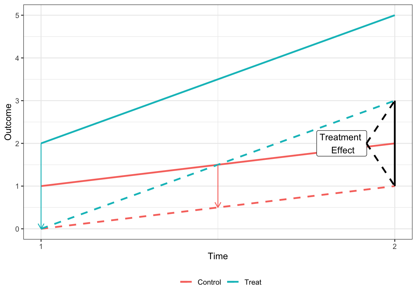
Basic DD Graph
Animations
Basic DD Graph, Animated
ATE Estimates with DD
Key identifying assumption is that of parallel trends
\[E[Y_{0}(1) - Y_{0}(0)|D=1] = E[Y_{0}(1) - Y_{0}(0)|D=0]\]
Estimation: Sample Means
\[\begin{align} E[Y_{1}(1) - Y_{0}(1)|D=1] &=& \left( E[Y(1)|D=1] - E[Y(1)|D=0] \right) \\ & & - \left( E[Y(0)|D=1] - E[Y(0)|D=0]\right) \end{align}\]
Estimation: Regression
\[y_{it} = \alpha + \beta D_{i} + \lambda \times Post_{t} + \delta \times D_{i} \times Post_{t} + \varepsilon_{it}\]
| Pre | Post | Post - Pre | |
|---|---|---|---|
| Treatment | \(\alpha + \beta\) | \(\alpha + \beta + \lambda + \delta\) | \(\lambda + \delta\) |
| Control | \(\alpha\) | \(\alpha + \lambda\) | \(\lambda\) |
| Diff | \(\beta\) | \(\beta + \delta\) | \(\delta\) |
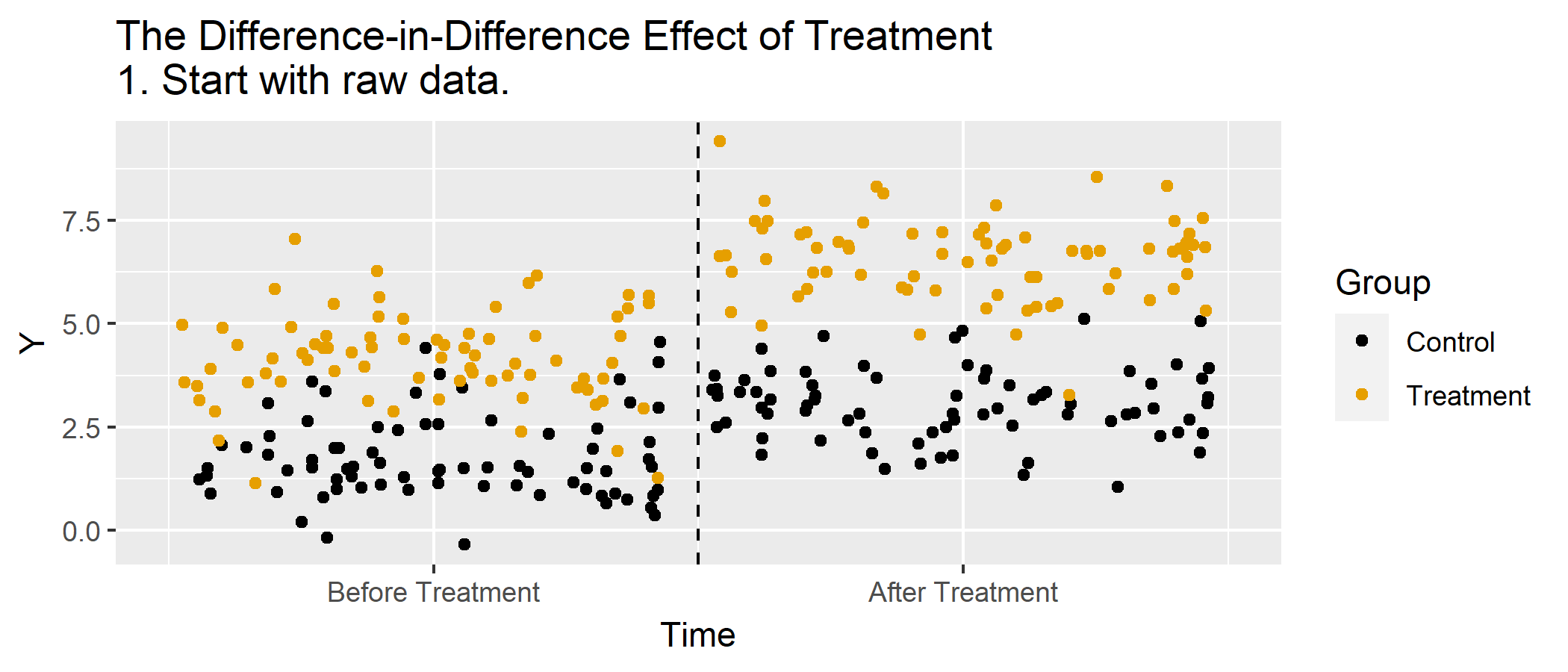
Simulated data
Mean differences
R Code
| Treated | Period | Mean |
|---|---|---|
| Control | Pre | 1.512192 |
| Control | Post | 3.010816 |
| Treated | Pre | 4.517785 |
| Treated | Post | 12.026116 |
Mean differences
In this example:
- \(E[Y(1)|D=1] - E[Y(1)|D=0]\) is 9.0152995
- \(E[Y(0)|D=1] - E[Y(0)|D=0]\) is 3.0055927
So the ATT is 6.0097068
Regression estimator
R Code
| (1) | |
|---|---|
| dTRUE | 3.006 |
| (0.028) | |
| tTRUE | 1.499 |
| (0.028) | |
| dTRUE × tTRUE | 6.010 |
| (0.040) |